
Version 11 and earlier help 
Historical help is preserved below with its original text, images, older screenshots and version references. These topics span earlier releases, so their screenshots and instructions can differ from version 12. For current instructions, start with version 12 help.
Contents 
- Known issues
- Antivirus programs
- Help: Apply theme to spreadsheet
- Best practices for responsive blocks
- Help: Pick a date with a Calendar widget
- Help: Use conditional formatting
- Help: Create and configure Responsive blocks
- Help: Create a theme with Theme Designer
- Help: Use both theme and Excel formatting
- Help: Design the web page for ALL your visitors
- Help: Edit and delete Responsive blocks
- Google Map
- Add the add-in to Excel manually
- The Barcode widget
- Customize and translate text
- Data Validation
- Dynamic dropdown menu
- The Worksheets tab
- Formatting the web page
- Help: Instant Testing
- Interactive charts
- Introduction to using widgets
- The Link Image widget
- Help: Live Preview
- The Print sheet
- The QR code widget
- Getting started
- Rules for input files
- The task pane
- Testing in Excel
- The Conversion Process
- The Excel ribbon menu
- Theme Preview
- User settings
- Translation overview
- Help: Use the basic widgets
- Visitor and conversion tracking
- The Messages tab
- Help: Hide rows or sheets with a widget
- Help: Introducing Responsive Design
- Help: Split web forms into two or more sections
- Help: Follow us in the Notification center
- Help: Open cells for user input
- Help: Scanning QR codes
- Help: Configure a web form's submit options
- Help: Convert to Node.js flavor
- Autosave form fields in browser storage
- Browser Storage
- Embed a Live Spreadsheet in WordPress
- Filling form fields from the link
- The Workbook tab
- How to change the regional settings in Windows
- How to obtain a Google Maps API key
- Install the WordPress plugin to import spreadsheets
- Manage Uploaded Spreadsheets in the WordPress Plugin
- Manually add a Google Maps API key
- Saving data in an online spreadsheet
- Secure login for Node.js
- Support guide for the WordPress plugin
- Advanced settings in version 8
- Help: The File Attachments widget
- The Excel ribbon menu
- The Workbook tab in version 8
- Upload a spreadsheet to WordPress
- The WordPress plugin to import spreadsheets
- Help: Use Offline Forms
- Help: Page fill color
- Publish to Cloud
- Collaborate with Real-time Sync, HTML flavor
- SpreadsheetConverter Real-time Sync Help
- Security concerns for Real-time Sync
- Help: Tips and tricks for web forms and submit
- Help: Use the basic widgets, iPhone/Android flavor
- Troubleshooting
- User-defined functions
Known issues 
Known issues 
This page contains a list of the known issues when using SpreadsheetConverter to convert Excel spreadsheets to live, calculating web pages.
Warning messages from Internet security programs 
All our files and computers are scanned for malware at all stages of production using the latest versions of industry-standard Internet security software which is updated automatically. All files available from our Download page are free of known malware. If your Internet Security software is flagging any part of our software as malicious, we urge you to contact us immediately. We are aware that e2o2.exe or ViewManager.exe sometimes get a “suspected” status, but so far these have all been false alarms. Read more on the help page for download and installation.
Old offline forms may cease to work 
In 2015 we introduced an offline forms feature built on a web standard called AppCache that is now being deprecated. We want you to be aware that depending on your web browser, AppCache-based offline forms may cease to work at some point in the future.
Our developers are investigating a new implementation. If and when such an implementation appears, you will need to upgrade to the then current version of SpreadsheetConverter and use it to re-convert your offline forms to use the new functionality.
Please contact our help desk if you have any questions regarding the future support for offline forms in SpreadsheetConverter.
Excel copies properties to new rows 
When you insert a new row in Excel, the default behavior is that certain properties are copied from the row above it.
In the example below, we are inserting a new row below row 23.
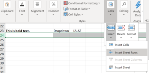
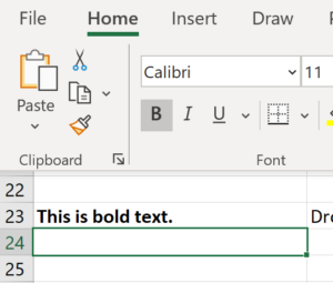
After we have inserted a new row 24, can see in A24 that the Bold font style attribute was copied from A23.
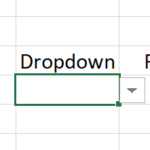
If we insert a new row below a dropdown menu, cell B24 below the dropdown in A24 also becomes a dropdown menu, as you can see from the small handle.
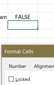
C24, the cell below the checkbox in C23, apparently did not become a checkbox. But something else happened to it, that is not easily recognized. Since C23 was unlocked, C24 quietly inherited the Unlocked attribute, which makes it an input cell if you use the Unlocked method of designating input cells.
Conclusion: Whenever you insert a new row in an Excel spreadsheet, some cell attributes will be copied from the cells in the row above the inserted row. You can try to avoid this by always selecting a row below an apparently empty row, but you may still run into issues because many “invisible” cell attributes like Bold and Unlocked remain even after the cell’s contents are deleted, and will be inherited by the new row without any visual feedback.
This is how Excel is designed, and there is nothing that SpreadsheetConverter can do about it.
Task pane issues with Windows 10.1903 
Windows 10 version 1903 introduced an error that caused the Excel task pane to stop working. The most apparent issue is that you cannot type anything into text fields in the task pane.
We have developed a circumvention for this problem. If you are affected by this error in Windows you should update to SpreadsheetConverter version 10.3 or later, or use a different version of Windows that doesn’t have the error.
Problems with multiple displays 
As Excel develops, new features are added that may be incompatible with old display drivers. This may result in apparent formatting errors.
In some systems, you may get a truncated display where some parts of the window are obviously missing or incomplete. The solution is to use the Optimize for compatibility setting described below.
Issues related to high-resolution displays 
Many modern tablets and laptops have displays with much higher resolution than their predecessors. Some people refer to this as having “a high dots-per-inch ratio”, or just “high DPI”. Excel gradually gets support for such “retina” screens, but you may still see scaling issues for add-ins like SpreadsheetConverter, especially when Excel is used with two or more monitors having different resolutions.
In some Excel versions, the text in the task pane may appear to be magnified and not proportional to the rest of the content on the screen.
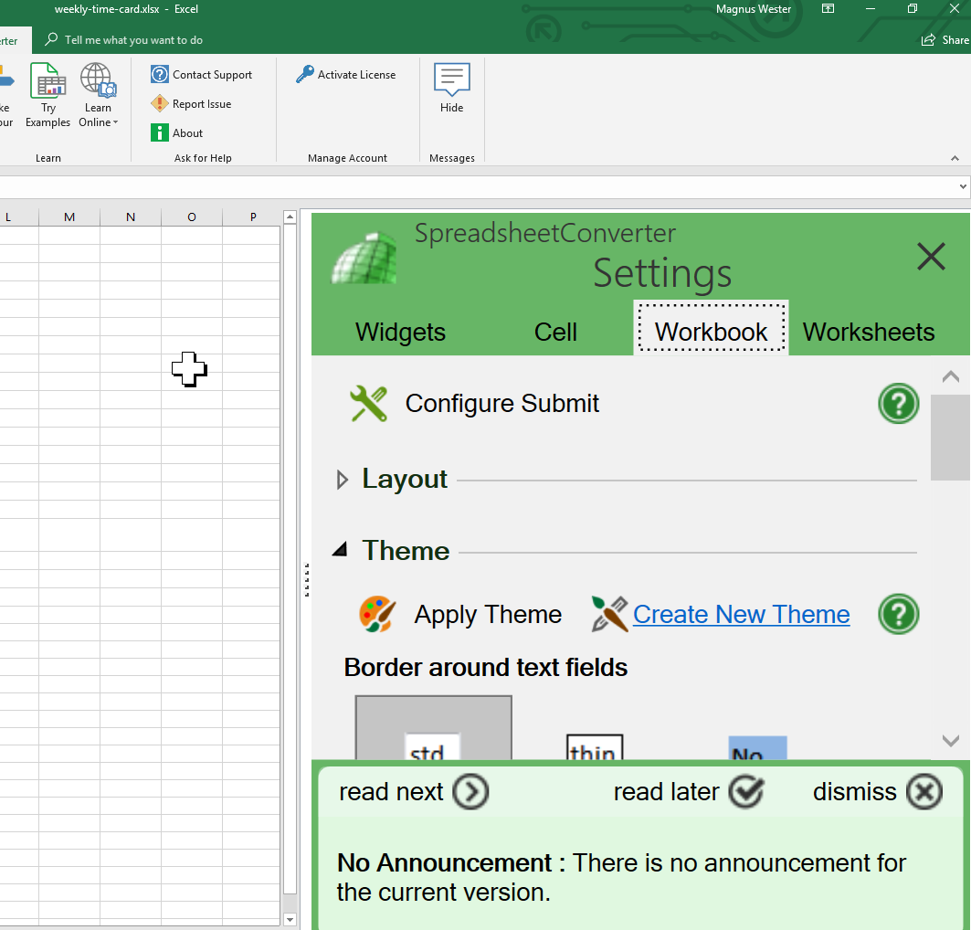
Other symptoms of these scaling issues are:
- The task pane contains large empty areas.
- When you click on SpreadsheetConverter buttons, menus or dropdown lists, the clickable area is very small, and the button or menu may appear not to work properly.
Use the setting “Optimize for compatibility” 
There is a simple circumvention for these problems. In Excel, go to File > Options > General > User interface options and select Optimize for compatibility.
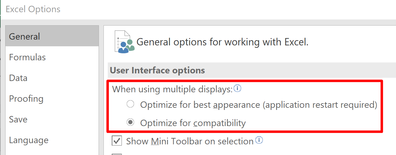
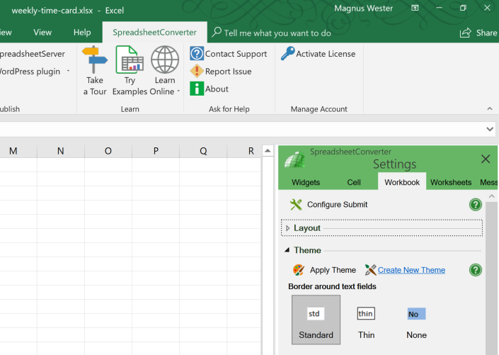
When using the Optimize for compatibility setting, Excel gets better at handling multiple screens with different resolutions. As you can see in the screenshot below, the SpreadsheetConverter task pane is now proportional to the rest of the screen.
Excel does not permit add-ins like SpreadsheetConverter to control the display scaling themselves. If your version of Excel doesn’t provide the compatibility mode for multiple displays, it will not properly support multiple displays with different resolutions, and you may see scaling issues like the ones described above until you upgrade Excel.
Cells that may contain both text and numbers 
When we designed SpreadsheetConverter we wanted to allow for extremely large spreadsheets, and still provide exceptionally fast response times on slow hardware. This forced us into a few minor compromises, of which one was that if you ever assign a text value to a cell, it is always treated like text. When you reference such a cell in your spreadsheet, it always returns a text string, even if this string only contains numbers.
- The cell contents will always be left-aligned, also when the string only contains numbers.
- In string comparisons, the operation compares the two strings character for character from left to right, so string values containing numbers may give unexpected results, e.g. ‘9’ > ‘10’ and ‘09’ < ‘9’.
- If you perform numeric operations with string values, the results may be unpredictable.
In spreadsheets that you intend to use with SpreadsheetConverter, you should clearly separate numeric variables from all other variables and never assign them any value that is not numeric.
A formula that returns either text or a number 
=IF($E2=0, "Error", ROUND(0.8/$H2,2))
SpreadsheetConverter will see that the formula may return the text Error and internally defines the cell as text, introducing the problems described above. To avoid this from happening, divide the functionality into two cells, one with the numeric value
=ROUND(0.8/$H2,2)
And another with the error indication
=IF($E2=0, "Error", "")
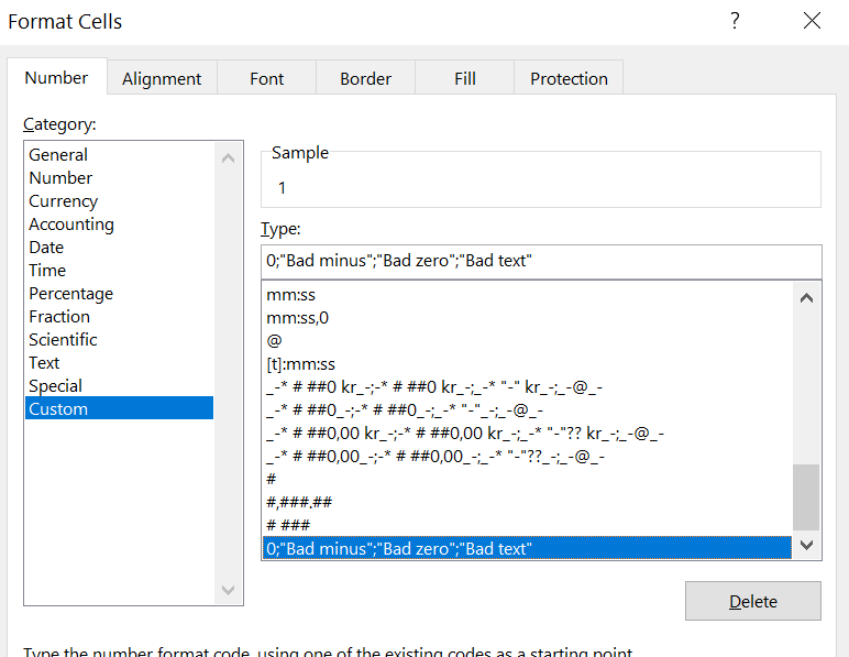
If you really need the error message to appear in the cell, perhaps for a table, you may be able to use a custom number format. A custom number format can have up to four sections of code, separated by semicolons. These code sections define the format for positive numbers, negative numbers, zero values, and text values, in that order.
<POSITIVE>;<NEGATIVE>;<ZERO>;<TEXT>
This allows you to display error messages instead of the cell contents for values that are positive when they shouldn’t be, or negative, or zero, or have a string value.
0;"Bad minus";"Bad zero";"Bad text"
The custom cell format above will only display positive numbers. All other values will be displayed as an error message. You define custom cell formats in the Format Cells dialog:
A formula that tests if a numeric cell is empty 
When you want to test if a numeric cell has no value, the correct way is to use a formula like
=IF(A1=0,"Empty", A1)
If you haven’t assigned any value to A1 yet, the formula above will fail, because SpreadsheetConverter regards empty cells as text strings, i.e. A1=””, and so the test will fail because A1<>0.
The obvious circumventions are:
- Never use empty numeric cells – always initialize all numeric cells with a default value of 0.
- Never use formulas that may assign text strings to numeric cells.
If you really, really must have a cell that contains both text and numbers, a safe test for it being empty is
=IF(OR(TRIM(A1)="",A1=0),"Empty",A1)
Another numerical/character problem that can be really challenging is zero suppression, which just happens to be the next topic.
Use the right way to suppress zeroes 
A common situation when cells may be forced to store both numbers and text (read more above) is zero suppression, where an otherwise numeric cell is set to blank if it is zero. Look at this worksheet for example:
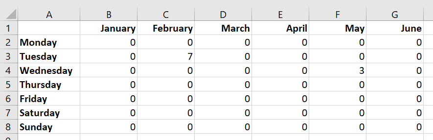
If there are many numbers on the screen, and many of them are zeroes, it can be hard to quickly grasp what a table is showing. Now look at what happens when we suppress the zeroes:
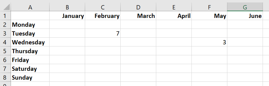
Many tables become much easier to read if we remove redundant information.
Inexperienced Excel users may try to suppress the zero values using an IF clause:
=IF(sum(jan_mon_1:jan_mon_5)<>0;sum(jan_mon_1:jan_mon_5);"")
This solves a small problem in a clumsy way, but also introduces a much worse problem – it is storing string values in numeric cells. Not only will this impact performance, it also risks introducing errors if non-numeric values are later used in calculations.
A better solution? Excel has many powerful cell formatting options. Get to know them, learn how to use them, and you will have much less need for circumventions like the if clause above. For numeric fields, a “0” in the formatting template is used to show the corresponding digit even if it is a zero, and “#” to show the number only when it is not zero. Zero suppression is built into Excel!
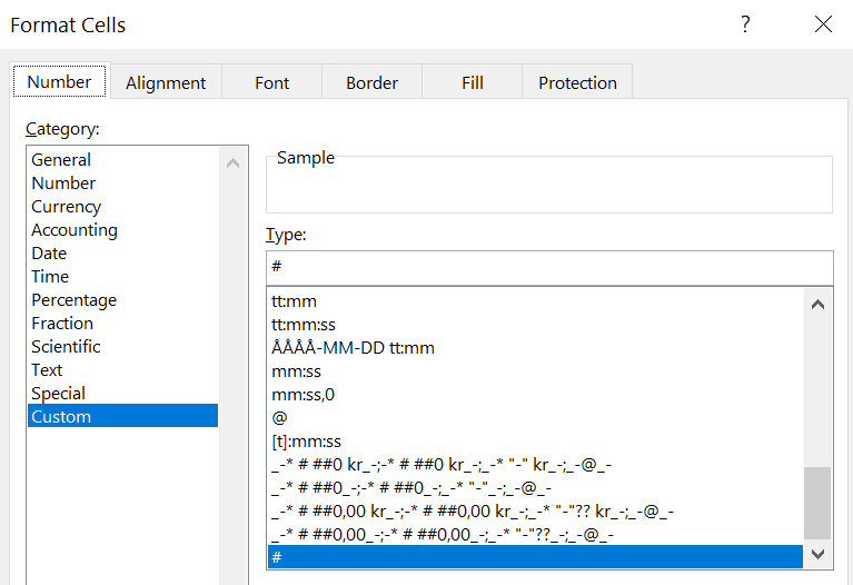
In the spreadsheet in the example above, we used the “#” custom format to suppress all the zero values in the table. It is a simple solution, but it may run into problems with currency symbols, thousand separators, and zero separators. If you want your numbers to be formatted like this:
$11,256.42
the “#” trick won’t help you, but Excel offers other ways to solve this. A custom number format can have up to four sections of code, separated by semicolons. These code sections define the format for positive numbers, negative numbers, zero values, and text values, in that order.
<POSITIVE>;<NEGATIVE>;<ZERO>;<TEXT>
You can use any advanced numeric formatting you like in the <POSITIVE> and <NEGATIVE> sections and then simply leave the <ZERO> section empty.
You can even use these code sections to create the following custom default cell format that can be used for all cells in a spreadsheet:
General;General;;@
If you apply this format to all cells in a spreadsheet, you will suppress all the zero values in all cells that don’t have their own number format set for them. All other text or numbers will have the same default formatting that they usually have.
If you like the idea, make it a habit to always apply this custom default cell format to all cells in new spreadsheets!
Use appropriate formulas 
A common problem in Excel is that it may not show you the true, entire numeric value of a cell. For example, if you enter the formula
=1/3
into cell A6, it will typically display as 0.333333. But the value actually has an infinite number of threes. So the statement
=IF(A6=0.333333, True, False)
will evaluate as False. Also, most computers actually perform decimal calculations as their equivalent binary calculations. This inherent approximation may lead to differences in precision, e.g. that a cell ends up with a value of 0.45000001 when you were expecting it to contain exactly 0.45. So, instead of the formula above, you should consider using
=IF(ABS(A6-0.333333) < 0.000001, True, False)
The same thing happens if you want to evaluate if a value is less than or greater than another value. If you get unexpected True situations using
=IF(A5 > A6, True, False)
it may be because one of the cells contains 0.45 but the other 0.45000001. To exclude this special case – where you prefer to consider the cells to be equal – use this formula instead:
=IF(AND(ABS(A5-A6) > 0.000001, A5 > A6), True, False)
If the numbers are close enough, the first part of the AND statement will not be True, and so A5 will not be considered greater than A6. You must use a “proximity constant” that is relevant for the numbers you are actually processing, in particular if you expect the cells to contain extremely high or low values.
Threaded comments are unsupported 
This issue requires you to know what version of Excel you are using. This information is available on the File > Account screen. 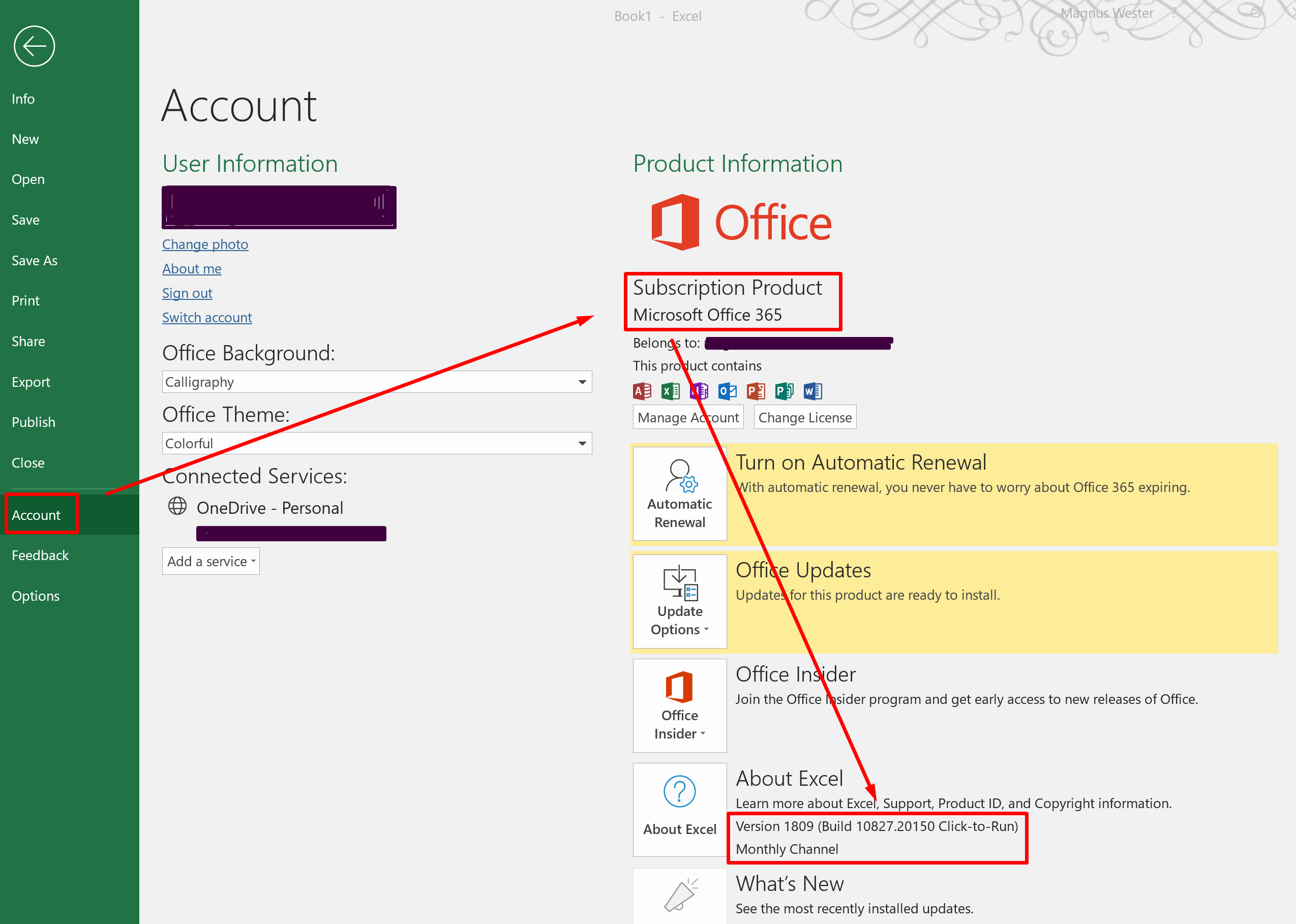 In Excel 365, version 1810, Microsoft introduced Threaded Comments. The new feature also became available in Excel 2016 version 16.17. With threaded comments, you can discuss a value or formula with other users of the same spreadsheet, just like in a chat or e-mail conversation. Notice the Reply… field in the screenshot below.

The old comments are now referred to as Notes. Notes look and work just like Comments have worked before.
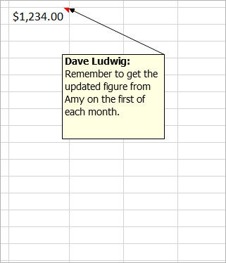
SpreadsheetConverter supports Comments from previous versions of Excel, and Notes from Excel version 1810 or 16.17, or later. If you use threaded comments in a spreadsheet that you convert with SpreadsheetConverter, the threaded comments will not be visible in the converted web page.
Restrictions for spreadsheet file name, size and content 
For your spreadsheet to convert gracefully into a properly formatted web page, it must follow certain rules. We have documented these in a separate help page about the restrictions for spreadsheet file name, size and content.
A conversion run never finishes 
If you start a conversion and the progress bar seems to get stuck around 32%, you may be using conditional formatting on a very large cell range, e.g. an entire column. This problem is easily solved, just apply conditional formatting to only those cells that actually contain data.
Cannot scan QR code to see the web page 
When the conversion is complete, you may be shown a QR code to scan with your mobile device. If the QR code doesn’t appear automatically, you can open the History List and scan it from there. If the web page doesn’t appear in your mobile device when you scan the barcode, and you get messages saying the website is unavailable, impossible to connect to or doesn’t respond, you may need to add an exception to the Windows Firewall. Read more in the online help for Instant Testing.
Empty sheets are not visible on the web page 
When you convert a spreadsheet where one or more of the worksheets are empty, the empty worksheets will not appear in the converted web page.
An error message appears instead of Google Maps 
New Google Maps may not appear as expected on your website. You get an error message saying Oops! Something went wrong. You likely have a problem with the Google Maps API key you use to show maps. Read the instructions on how to solve this.

Handling forms 
“Unresponsive script” message from Mozilla Firefox 
When a user with the Firefox web browser presses Submit on a form that contains a chart, and you are using the Advanced Submit Service to deliver the submitted form also in PDF format, the user may get the following error message from Firefox: 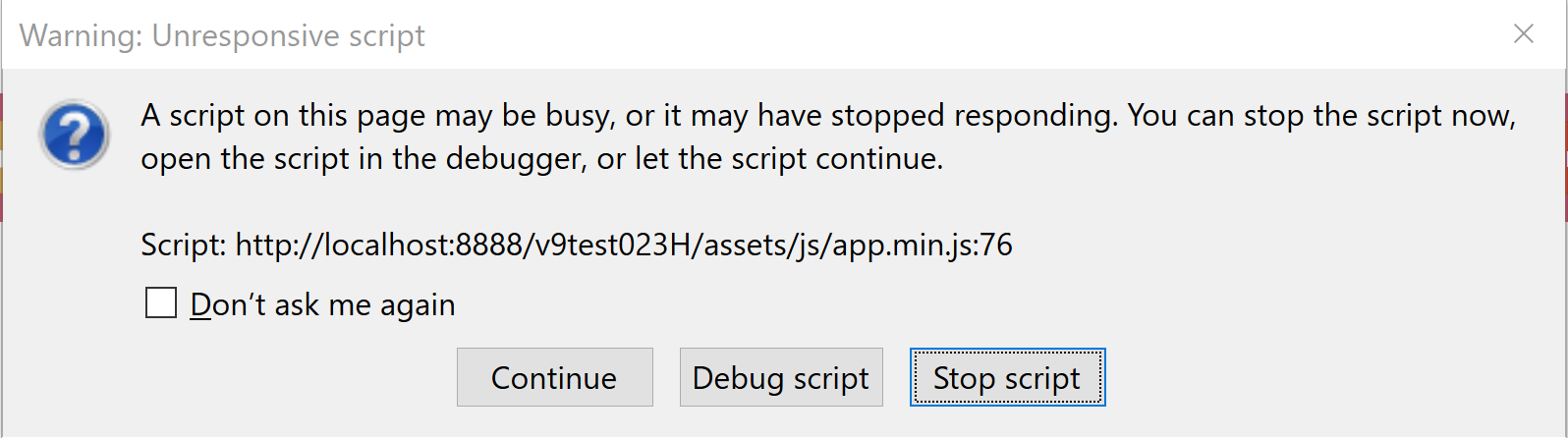 The process of preparing the PDF file is partially taking place in the browser, and on slower computers the required processing may take so long that it exceeds the built-in script time-out in Firefox. The best way to verify this is to test the form with a different web browser. If the form can be submitted without errors using a different browser, you have the situation described above. The simplest solution is just to press Continue if the message appears after submission of a form. If the message becomes a problem you may suggest that the user reads Mozilla’s help page on how to increase the script time-out in Firefox to 20 seconds. Increasing the time-out has no negative effect except that it takes slightly longer for Firefox to detect other situations when a script has stopped responding – but this is not a common problem.
Delivering forms via e-mail 
Our Free and Advanced e-mail services run on secure web servers, where incoming form submissions are saved. For each new form we receive on your behalf, we send an e-mail to one or more e-mail addresses designated by you, with the contents of the submitted form. E-mail is built on a store-and-forward architecture, and in the worst case, an e-mail from our server may have to pass multiple servers before it reaches its recipients. The e-mail infrastructure is beyond our control and there is simply no way for us to guarantee that you will get all the e-mails we send you. With the Advanced Submit Service, you get a personal login to our forms database. We recommend that you periodically use this login to monitor our server manually for new form submissions, in case the corresponding e-mails have been discarded by the e-mail infrastructure. The risk of losing e-mails increases when you use File Attachments. We recommend that you use our Secure Delivery feature to have the e-mail contain just a link to the form instead of the form’s full contents with attachments.
Old e-mail clients 
The e-mail we send you for a submitted form uses industry-standard formatting and markup. Some e-mail clients may not provide full support for current standards. In this case, hidden sheets may be visible in the e-mail, the formatting may not be perfect etc.
Antivirus programs 
Antivirus programs 
Some Internet Security suites may interfere with the normal operation of SpreadsheetConverter. This page documents the symptoms and possible actions you can take.
There are many “Internet Security” products for safe browsing by companies such as Symantec/Norton, Kaspersky, McAfee, Trend Micro and Bitdefender. Some of these products may incorrectly assume that SpreadsheetConverter contains malicious code.
- There are no known security vulnerabilities in SpreadsheetConverter.
- All our files and computers are scanned for malware at all stages of production using the latest versions of industry-standard Internet security software which is updated automatically.
- All files available from our Download page are free of known malware.
- You can safely download, install and use the program.
Traditionally, antivirus programs use known “signatures” of malicious files. This technique cannot detect new and unknown malware which may be working its way around the Internet. In order to provide additional protection, most Internet security software also uses advanced techniques to warn their users of unusual behavior. Such “deep-scan” or “heuristic” features are typically much less exact than traditional signature matching and can result in false alarms which may affect any legal, malware-free software.
We sometimes get false warnings for two specific programs, e2o2.exe and ViewManager.exe. When you use our Excel add-in we would prefer to run these programs close to Excel but unfortunately this may lead to memory leaks that are beyond our control. Therefore they are currently run as separate processes using the Windows Command Prompt. This is a short-term solution that solves a lot of problems but creates a few others. The worst is that some Internet Security products incorrectly assume that these programs are piggy-back, “trojan” attachments of malicious code.
If your Internet Security software is flagging any other part of our software as affected by malware, we urge you to contact us immediately. But so far, all warnings that e2o2.exe or ViewManager.exe are behaving strangely or get a “suspected” status have been false alarms. We regret any inconvenience this may cause you and we are working on a long-term solution for this.
If your Internet Security software is incorrectly flagging e2o2.exe or ViewManager.exe as malicious, you should add these programs to the “known to be safe” or “exclude from scanning” list, or disable the entire antivirus program when you download, install or use SpreadsheetConverter.
Avast 
The Internet Security suites from Avast are highly rated and we encourage you to use them. If you are the first to install a new version, you may receive a message that e2o2.exe and/or ViewManager.exe have been sent to the Avast labs for examination. This is perfectly normal and the program will usually be approved in just a few minutes. Otherwise, Avast has no known issues with SpreadsheetConverter.
AVG 
The Internet Security suites from AVG are highly rated and we encourage you to use them. They have no known issues with SpreadsheetConverter.
Avira 
The Internet Security suites from Avira are highly rated and we encourage you to use them. They have no known issues with SpreadsheetConverter.
Bitdefender 
The Internet Security suites from Bitdefender are highly rated and we encourage you to use them. However, it seems to be falsely assuming that any program run as a separate process is a so-called trojan. In our case, it does not permit e2o2.exe to run, even though this is a completely harmless program that has been used safely in thousands of installations since 2002. If you use Bitdefender, you need to turn off all switches including Safe Files before you press the Convert button on the SpreadsheetConverter menu in Excel.
If you happened to start a conversion without disabling Bitdefender first, it will have deleted some of the files that are required for SpreadsheetConverter. To correct this, turn off Bitdefender, start the installation program again and select the Repair option.
Comodo 
The Internet Security suites from Comodo are highly rated and we encourage you to use them. They have no known issues with SpreadsheetConverter.
Dr. Web 
The Internet Security suites from Dr. Web are highly rated and we encourage you to use them. They have no known issues with SpreadsheetConverter.
ESET 
The Internet Security suites from ESET are highly rated and we encourage you to use them. They have no known issues with SpreadsheetConverter.
F-Secure 
The Internet Security suites from F-Secure are highly rated and we encourage you to use them. They have no known issues with SpreadsheetConverter.
G Data 
The Internet Security suites from G Data are highly rated and we encourage you to use them. They have no known issues with SpreadsheetConverter.
Kaspersky 
The Internet Security suites from Kaspersky are highly rated and we encourage you to use them. They have no known issues with SpreadsheetConverter.
Malwarebytes 
The Internet Security suites from Malwarebytes are highly rated and we encourage you to use them. They have no known issues with SpreadsheetConverter.
McAfee 
The Internet Security suites from McAfee are highly rated and we encourage you to use them. They have no known issues with SpreadsheetConverter.
Microsoft Defender 
Microsoft Defender offers built-in protection for your Windows devices. It is highly rated and we encourage you to use it.
During installation, you may get this message:
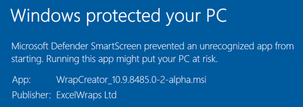
This is normal and you should click on Run anyway.
Norton 
The Internet Security suites from Norton are highly rated and we encourage you to use them. They have no known issues with SpreadsheetConverter.
Panda 
The Internet Security suites from Panda are highly rated and we encourage you to use them. They have no known issues with SpreadsheetConverter.
Sophos 
The Internet Security suites from Sophos are highly rated and we encourage you to use them. They have no known issues with SpreadsheetConverter.
Symantec 
The Internet Security suites from Symantec are highly rated and we encourage you to use them. They have no known issues with SpreadsheetConverter.
Trend Micro 
The Internet Security suites from Trend Micro are highly rated and we encourage you to use them. They have no known issues with SpreadsheetConverter.
TrustPort 
The Internet Security suites from TrustPort are highly rated and we encourage you to use them. They have no known issues with SpreadsheetConverter.
Webroot 
The Internet Security suites from Webroot are highly rated and we encourage you to use them. They have no known issues with SpreadsheetConverter.
Help: Apply theme to spreadsheet 
Apply theme 
Download the stylesheet from Theme Designer, import it into SpreadsheetConverter and apply the theme to your web pages.
Theme Designer allows you to set a number of visual attributes for your web calculator and save them as themes that can be applied to one or more spreadsheets. After you’ve created a theme, you must download it to SpreadsheetConverter and select it for your spreadsheets.
This Help page shows you how to import a modified theme to Excel and use it when converting your spreadsheets for the web. Before you continue, you need to be familiar with the basic concepts presented in the help page on how to create a theme with Theme Designer.
Download the theme 
Click on the Download button in Theme Designer to download the theme you have just created. The file is in CSS format (Cascading Style Sheet) and the file name always ends with -ssc-min.css.

Apply the theme to a spreadsheet 
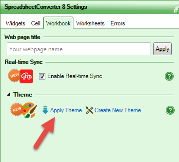
Click on Apply Theme in the Theme section of the Workbook tab to set a theme for the current spreadsheet.
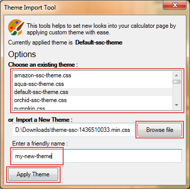
Click on Browse file (see below) and select the CSS file you just downloaded from Theme Designer. Enter a friendly name that helps you remember the theme, without spaces, please.
You can also select one of the already downloaded themes in the list.
Press Apply Theme.
Generate a web page with the theme applied 
Select the flavor you want and convert the spreadsheet. When you open the web page in a web browser it has the visual appearance defined by the theme.
Test different designs with ThemePreview 
The ThemePreview toolbar allows you to change the theme directly in the web browser, to see which design works best for your calculator or form. It also allows you to change a few settings for the web page that can’t be stored in the theme.
Tips and tricks 
Updating a theme 
Theme Designer retains its most recently used settings. If you want to iteratively tailor a theme further you can just continue where you left off and download the theme file again and again until you are satisfied with the results.
Renaming, deleting or replacing themes 
The theme’s stylesheet is physically packaged together with each calculator when you convert it to web format with SpreadsheetConverter. Each web page will only use the stylesheet it was packaged with during conversion. Renaming or deleting themes has no effect on previously converted calculators. Also, replacing a theme with new settings will not affect existing calculators that use the theme until you convert them again.
Removing a theme from a calculator 
To remove any previously applied theme from a calculator, select default-ssc-theme.css in the list. This gives your web page the same neutral design as it had before any theme was applied.
Best practices for responsive blocks 
Best practices for responsive blocks 
This page contains tips and tricks to help you become successful with responsive blocks. We hope this collection of best practices will help you create the best possible responsive designs for your calculator or form.
Before you separate a spreadsheet into responsive blocks you may want to prepare it a bit for the new challenge.
With responsive design, one or more responsive blocks will be placed side by side on the screen until the whole width of the screen has been utilized. The first block that doesn’t fit at the end of the current row of blocks will instead appear first in a new row of blocks.
Portrait blocks are better than landscape 
Already from the start, the screen of your mobile device is probably less wide than that of your office computer. To make matters worse, many mobile devices are most conveniently used in their portrait orientation, i.e. with the shortest side up, while most office computers typically operate in landscape orientation with the longest side of the screen at the top.
When you design spreadsheets for portrait-mode devices, you may have to rethink the entire design of the sheet. Try to divide the contents of the spreadsheet into rectangular areas with portrait orientation. The contents of each block should be as independent as possible of other things in the spreadsheet since each block may fill the entire screen on smaller devices. To see anything outside the currently visible block, the user will have to scroll up or down.
On the other hand, if you try to show too many spreadsheet columns at the same time on a small screen in portrait mode, they will become zoomed out and difficult to read. Try to make your blocks contain as few spreadsheet columns as possible.
Don’t create horizontal information structures in your spreadsheet if you can avoid it.
Do repeat the row headings for every data column to increase the readability on narrow screens where only one data column may be shown at a time.
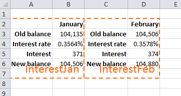
Responsive blocks cannot overlap 
Keep in mind that responsive blocks are rectangular cell areas that cannot overlap.
Don’t include any cell in the spreadsheet in more than one responsive block.
Do move things about in the spreadsheet if necessary to create non-overlapping rectangular areas.
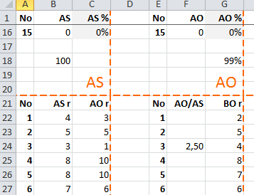
Blocks always appear in the same order 
Regardless of the screen width, responsive blocks always appear on the screen in the same sequence as in the original spreadsheet when reading from left to right, going down.
Before you define the responsive blocks for a spreadsheet you may want to redesign it so that the order of the blocks will be natural also for users of mobile devices that view the calculator’s responsive blocks in a rearranged form.
Don’t use arrows to point to things in the spreadsheet. With responsive blocks, the section you thought would be to the right may instead appear below the current.
Do put the most important or summary information in the left-most, upper-most responsive blocks, so that it appears first on all devices.
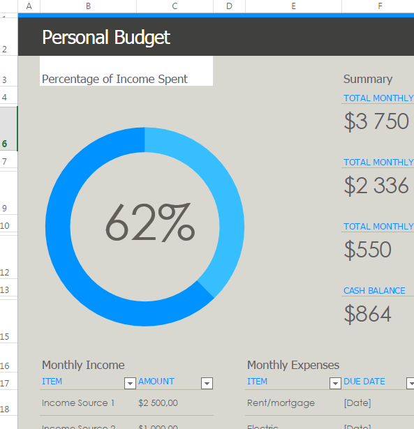
Try to keep white-space to the right 
Some responsive blocks contain more spreadsheet rows than other blocks, making them longer. When two or more blocks appear side-by-side, it often looks best if the left-hand block is the longest. Having a lot of white-space in the left part of the screen can look strange in countries where people read from left to right.
Don’t assume that the blocks will relate to each other the same way on small screens as they do on your office computer.
Do test your spreadsheet on both phones and tablets to see how white-space appears as you scroll through the worksheet.
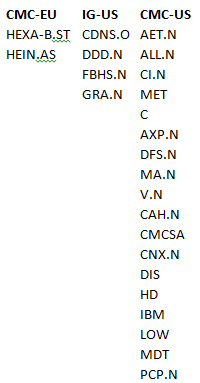
Tables are tricky 
One of the main purposes of responsive design is to avoid horizontal scrolling. For tabular data, this can be impossible to achieve. Let’s say you have a table of financial data per month. We currently do not offer a way to automatically decompose such a table into responsive blocks without losing the row headings as you scroll to the right.
Don’t create a single responsive block for a large table. Narrow screens will zoom out for all columns to fit, and the text will be impossible to read.
Do move every complex table to a separate worksheet, without defining any responsive blocks for it. In this case, responsive design will not be enabled for the worksheet. Users can scroll horizontally to see the entire table.
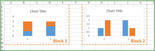
Use a separate block for each chart 
Charts are special objects and making them responsive requires special attention. Try to use a separate responsive block for each chart so it does not mix with other charts or texts.
Don’t
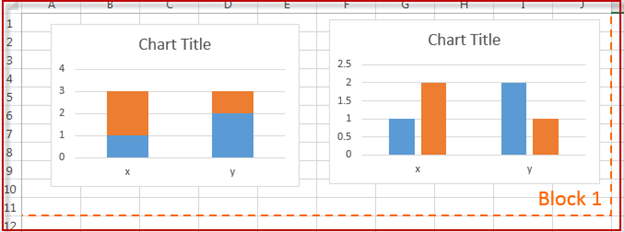
Do 
Put the headings with the chart or data 
If you have a heading on the top of a chart or data column, put it inside the same block as the chart or data. Otherwise, the heading may be separated from the chart or data.
Don’t
If you separate the heading of each chart into 2 blocks, then the heading of the second chart will move below the heading of the first chart.
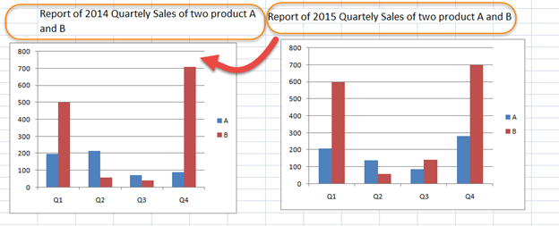
Do
Define the blocks like this instead:
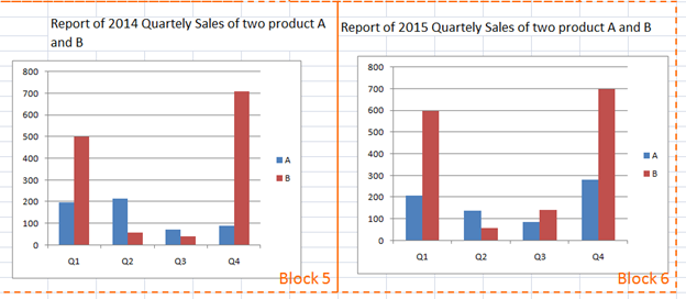
Place charts and maps in merged cells 
When you use graphical items like charts, maps and some of the widgets, it is easy to just drag the placeholder to the right spot on the sheet. In many cases, the resulting web page will look fine anyway. This is thanks to Excel’s graphical layers, that allow you to position stuff freely on top of a spreadsheet.
Don’t just float the chart on top of the worksheet. As you can see in the screenshot below, the chart is not properly enclosed in a single cell.
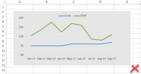
With responsive design, it may be difficult to place a chart or map in exactly the right position on the web page just based on where you put the placeholder in the graphical layer. To ensure a correct result with responsive design, always place charts, maps and graphical widgets in their own cell.
Do merge cells to make room for each chart or map. In the screenshot below, the cells A2:E13 have been merged to become a much more reliable home for the chart.
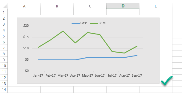
Border lines and block boundaries 
Border lines between columns in spreadsheets may look like they are shared by the two columns, but they aren’t. Column A may have a right border or columns B may have a left border. To you it looks the same but to Excel it’s two different things.
When you define responsive blocks with border lines along the edges of the block, Excel may consider the borders part of another responsive block than you do, and so the blocks appear for the wrong responsive block.
Don’t use border lines at the boundaries of responsive blocks.
Do use other visual signals like background colors to visually separate blocks from each other.
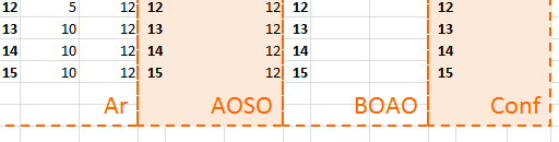
All or nothing is responsive 
In a responsive worksheet, all active cells must belong to a responsive block.
Don’t forget any active cells when you define the responsive blocks.
Do accept that some worksheets just cannot be made responsive. For some sheets, horizontal scrolling is the only way to go.
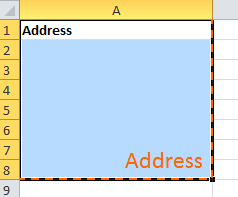
A responsive block must have at least two rows or columns 
We don’t like restrictions but we do have a few. You may be tempted to create a responsive block that contains only one cell. This is usually a large merged cell that you thought you could use as a separate Responsive block. And here comes the restriction: you can’t. It causes Excel to lose the column width.
Don’t create a responsive block that contains only one cell.
Do include some extra cells in every responsive block that contains a single cell. Just add a cell above with a text heading and it will work fine.
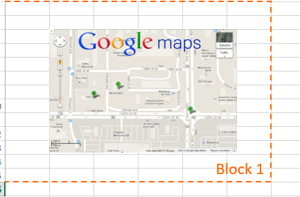
Use margins for maps or images 
Add an extra column to the left- and right-hand side of every Google map. If you don’t, mobile users may become unable to scroll through the web page – they will re-center the map instead.
Don’t let maps fill the whole screen. The map will just follow the users’ finger movements on the screen to a new location, and users can no longer scroll through the webpage.
Do use margins also for responsive blocks that only contain a map or an image. The margins provide a space for users to drag their fingers when scrolling.
How do I design a spreadsheet to look good as a web page ? 
Read our comprehensive design guide to learn how to design web calculators for a global, mobile audience:
- A large part of your users will be using their phones to use the web page.
- Put the caption on top of each field, not to the left of it.
- Arrange the sections of the calculator or form below each other, or on different tabs.
- For wider examples, you must use responsive design to make the example fit also narrow screens.
- As a desktop user, you may love to analyze data in wide tables with countless columns. This doesn’t work well on phones. You have many options.
- Always test all your calculators with your own phone.
- Assume your calculator or form will be used by an international audience.
- Your calculator may need to handle both metric and US customary units.
- Learn more about the differences in the formatting of date, time and numbers.
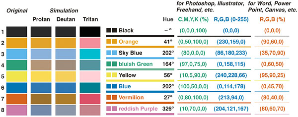
- Use only colors that are as far away from each other as possible, using colors that are unambiguous also to colorblind persons.
- Use the table in the design guide.
Help: Pick a date with a Calendar widget 
The Calendar widget 
To make it easier for your visitors to enter a date into your form, use a Calendar widget.
If you need your visitors to pick a date in a form, use the calendar widgets. This makes it easier to locate the right date, and reduces the risk of errors considerably. You can use formulas to calculate a default date.
Calendar widget 
Calendar widgets make it much easier for the user to pick the right date. It also makes it easier to count from one date to another. The widgets ensure that any date picked from the calendar is valid, and formats it correctly for the recipient of the electronic web form using the regional settings.
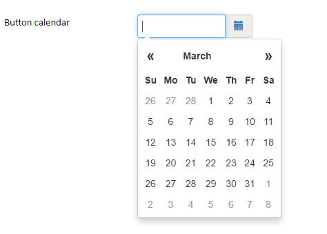
The calendar automatically uses the developer’s regional settings for the names of months and days. If your regional settings are for Swedish, your calendar looks like this instead:
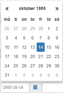
You may need to change your regional settings before you convert the spreadsheet to a web page. Example: If you normally use the regional settings for French (Canada), but the web form you are developing is in English (Canada), you must switch to the corresponding regional settings before the conversion and you may also have to restart Excel.
When the user selects a date in the calendar, it appears in the widget cell, formatted according to your computer’s regional settings. The calendar may be positioned at a default date, e.g. today + 30 days. If there is a default date, it is visible in the date field already from the start.
Excel serial numbers 
Excel stores dates as sequential serial day numbers so that they can be used in calculations. By default, January 1, 1900, is serial number 1, and January 1, 2008, is serial number 39448 – because it is 39,447 days after January 1, 1900. The date returned by the calendar widget is always in the form of an Excel serial number.
Options for the Calendar widget 
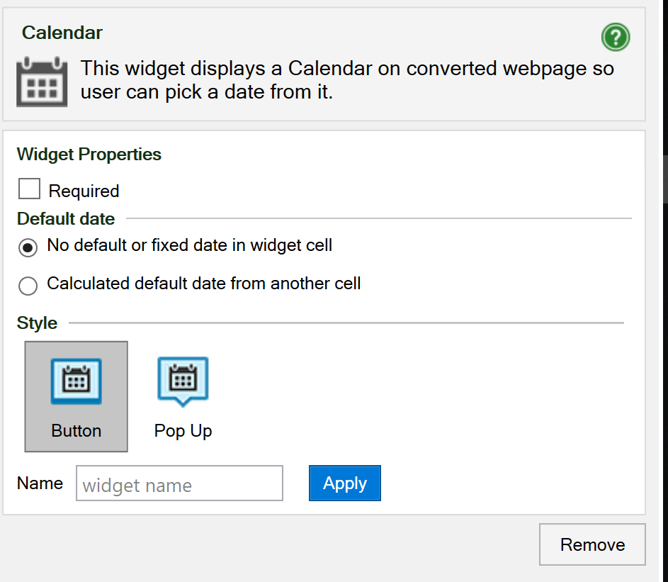
Required 
A Required field requires input from the user. This option is mainly used for electronic forms, where a form must contain a minimum of information to be meaningful. For Calendar fields, a Required date cannot be empty – a designated date must appear in the widget cell. If the widget cell is empty, no date has been selected, and the form cannot be submitted.
Default date 
If you don’t provide a default date, the calendar will position itself on the user’s current date but not select it. If you have selected the Required option, it is not fulfilled until the user explicitly clicks on a date to select it.
If you do provide a default date for a Calendar widget, your proposed default will appear in the field and the calendar will position itself on the default date, and it will be selected. To select a date other than the default, the user must select a different date in the calendar. If you have selected the Required option, it is always fulfilled when there is a default date, unless the user empties the date field or types an invalid date into it.
The default date assignment order 
The default date can come from one of five sources. The assignment occurs in the order below, using the first valid date that is eligible. We call this the default date assignment order.
- The most recent value saved by a Real-time Sync session with the same key.
Real-time Sync is a feature that allows multiple users to edit the same form or calculator simultaneously. With Real-time Sync, the contents of a form become persistent. You may return to a form years later and it will still contain the values from the most recent editing session. - A date set by the query string for the link that invoked the form.
You can assign a value to a date field from the link. You can either use an Excel serial number, e.g. /form.htm?built_date=20376 or your regional date format, e.g. /form.htm?built_date=10/14/1955. Read more about filling form fields from the link. - A calculated default date from a formula cell.
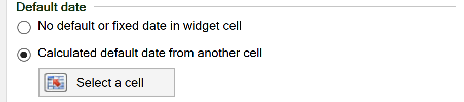
If you select to assign a Calculated default date from another cell, you must select a formula cell in the spreadsheet from which the calculated default date is taken. When the Select another cell window appears, just select the formula cell (or type its cell reference into the window) and press OK.
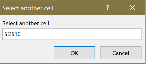
In the formula cell, D10 in the example above, you can calculate the default date using any suitable formula, e.g. =TODAY()+7. The formula cell must contain a valid date in the form of an Excel serial number. For clarity, you may want to assign a date format to the formula cell, so that you can see what date it is returning to the Calendar widget. If you wish to provide a dynamic date as pre-filled input to the date calculation formula, you can use a hidden cell in the spreadsheet, e.g. “/form.htm?ship_on_default=20376”, and then your date calculation formula can pick this up and use it when selecting the default date, e.g. “=IF(OR(ship_on_default = “”, ship_on_default > 0), ship_on_default, TODAY()+30)”.
- The most recently used date from browser storage.
If Browser Storage is enabled for a form, all form contents are saved in the browser. When the same form is opened again, it is prefilled with the data from the previous form submission in order to save time. Read more about Browser Storage. - A fixed default date typed into the widget cell.
You can provide a fixed default date simply by entering it into the widget cell in the source spreadsheet.
Regardless of how the default date is set according to the assignment priority above, the calendar will position itself on the default date, and it will be selected. With a valid default date in the cell, Required is always fulfilled.
Calendar style 
There are two calendar styles:
- The Button calendar is represented by a plain text field with a button in the form. The Full calendar appears when you press the button. The calendar disappears again when the user selects a date in the calendar.
- The Pop-up calendar appears as a plain text field in the form. The Full calendar appears when you place the cursor in this field. The calendar disappears again when the user selects a date in the calendar.
Widget name 
Name your widgets if you want to pass data into them from the link to the form (see above). For electronic forms, it makes it much easier to process the form if all input fields have names. You can name your fields in the widgets or give them cell names in Excel. Widget names can start with numbers or an underscore, which may be required when integrating with products like Salesforce.
Remove the calendar widget 
Click on the Remove button to remove the calendar widget from the widget cell.
Hiding a calculated default date 
As you can see in The default date assignment order above, you can use a separate formula cell to calculate a default date for the Calendar widget. You can use the same technique to put a fixed timestamp into each form, e.g. using the function =NOW().
In both cases, the cell contains a formula and will be locked for user input. It is not hidden by default, however. To hide a calculated date, insert a Utility widget into the formula cell and select Make hidden field. Even if you hide the default date in the web page, it will be included with the other form fields when the form is submitted.
Help: Use conditional formatting 
Conditional formatting 
With SpreadsheetConverter, you can use most of Excel’s conditional formatting in the converted web page.
SpreadsheetConverter supports most of the conditional formatting rules in Excel. If your spreadsheet has conditional formatting rules, the same rules will be applied in the live web page.
With conditional formatting in Excel, cells can change color or other visible properties depending on their value. If you use conditional formatting in your Excel spreadsheet, these rules are also applied when the spreadsheet is converted to a web page.
SpreadsheetConverter supports slightly different conditional formatting rules depending on the version of Excel it is used with. Some specific features of conditional formatting are currently unsupported:
- Above/Below standard deviation
- Duplicate/unique
- Top/bottom n percent
- Applying conditional formatting to a huge cell range, e.g. an entire row or column, like $B:$B
- Midpoint axis for negative values and border colors in Databar
- Icon-sets
Example 
To demonstrate this function, we created a web version of the popular Sudoku game using just a spreadsheet.
Sudoku converted to a webpage with conditional formatting
Known issues 
- If you use conditional formatting on a web form that is submitted, the conditional formatting will not be carried over to the formatted web form in the e-mail you receive.
Help: Create and configure Responsive blocks 
Responsive blocks 
In this Help page, we will show you how to split a spreadsheet into responsive blocks that wrap nicely on all screens.
If you are new to responsive design, you may first want to read the introduction to responsive design.
Before you create your first responsive spreadsheet, we suggest you read our best practices for responsive blocks to avoid the most common mistakes.
Define the responsive blocks 
This part of the tutorial shows you how to define the responsive blocks in your spreadsheet.
Open the settings 
Open the Responsive blocks settings from the ribbon.
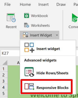
Add New 
Click on the Add new button.
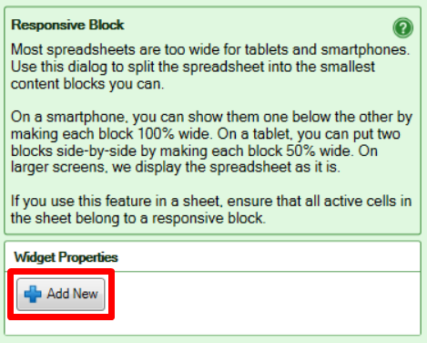
Select Range 
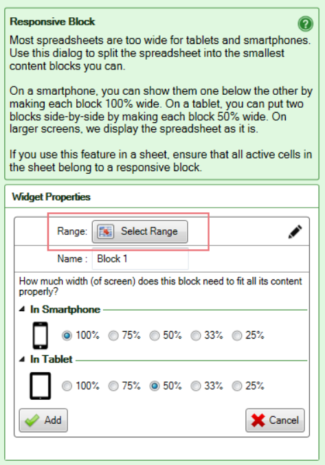
This opens the widget properties panel, in which you select the cell range for the first block. Click on Select Range.
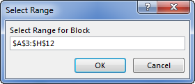
When the Select Range box appears, place the cursor in the input field and type the coordinates for the block or drag the cursor diagonally across the cell range.
Block Name 
Give the block a name that makes it easy to understand its function in the spreadsheet, and its contents.
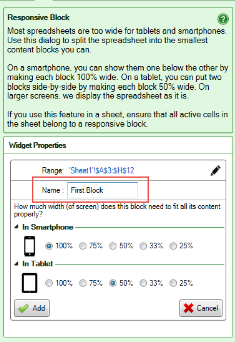
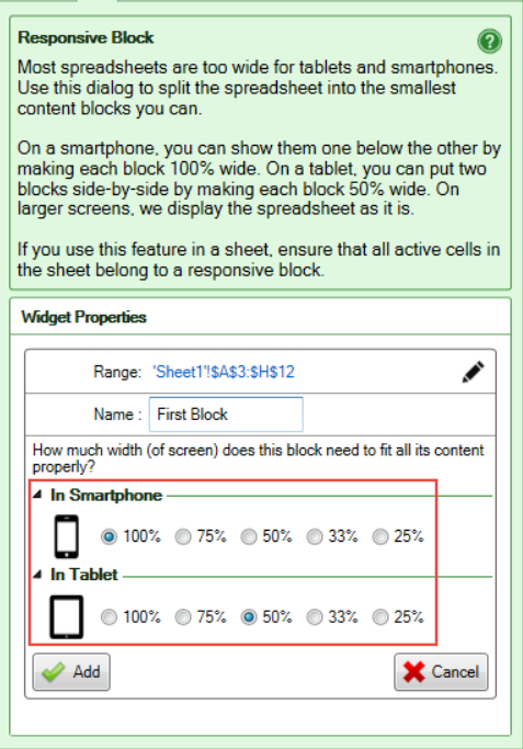
Block Width on phone and tablet 
Specify how much of the screen width to use for the block. There are separate settings for phones and tablets.
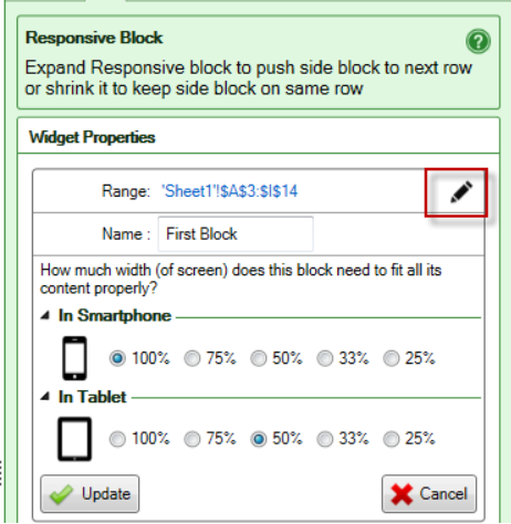
In the below screenshot, the block will use 100% of a phone screen but only 50% on a tablet. This gives room for additional blocks to the right if they use 50% or less of the screen width.
Preview your block definitions 
This part of the tutorial shows you a preview of how the screen will be used on a phone and tablet.
The orange visualizer 
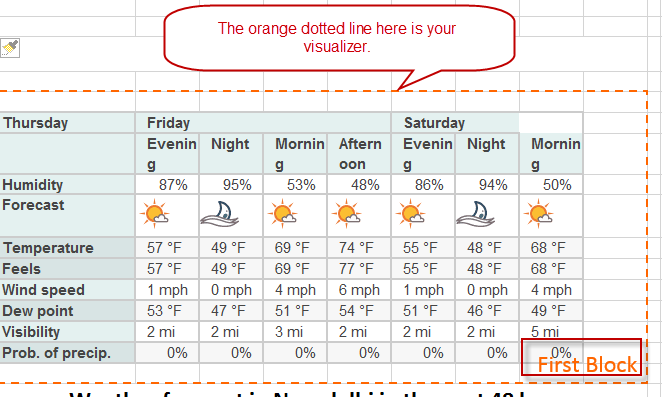
Click the Add button. An orange dotted line appears in your spreadsheet to visualize the responsive block. At the bottom of the visualizer, you see the name of the block. Please do not directly edit the visualizer graphic.
The Preview tool 
The Preview section shows you how the blocks you have created will appear on phone screens. Since the width was set to 100%, each block fills the screen so only one block at a time is shown.
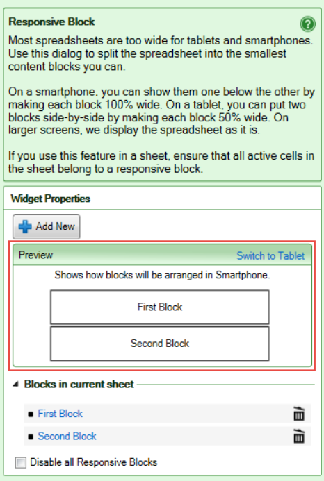
If you want to see how your blocks will fill a tablet screen, press Switch to Tablet. Since each block only requires 50% of the screen, they now fit beside each other.
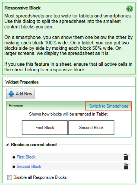
Continue defining responsive blocks until all active cells in the spreadsheet belong to a responsive block.
Convert your spreadsheet 
Press Convert in the ribbon to convert the spreadsheet for the selected target environment.
Adjust the window width 
You don’t need a tablet or smartphone to verify your responsive design. The layout is responsive already on your laptop and will automatically adapt to any change to the width of your browser window. Just make the browser window more narrow and you will see how the responsive blocks automatically reposition themselves for the new window width.
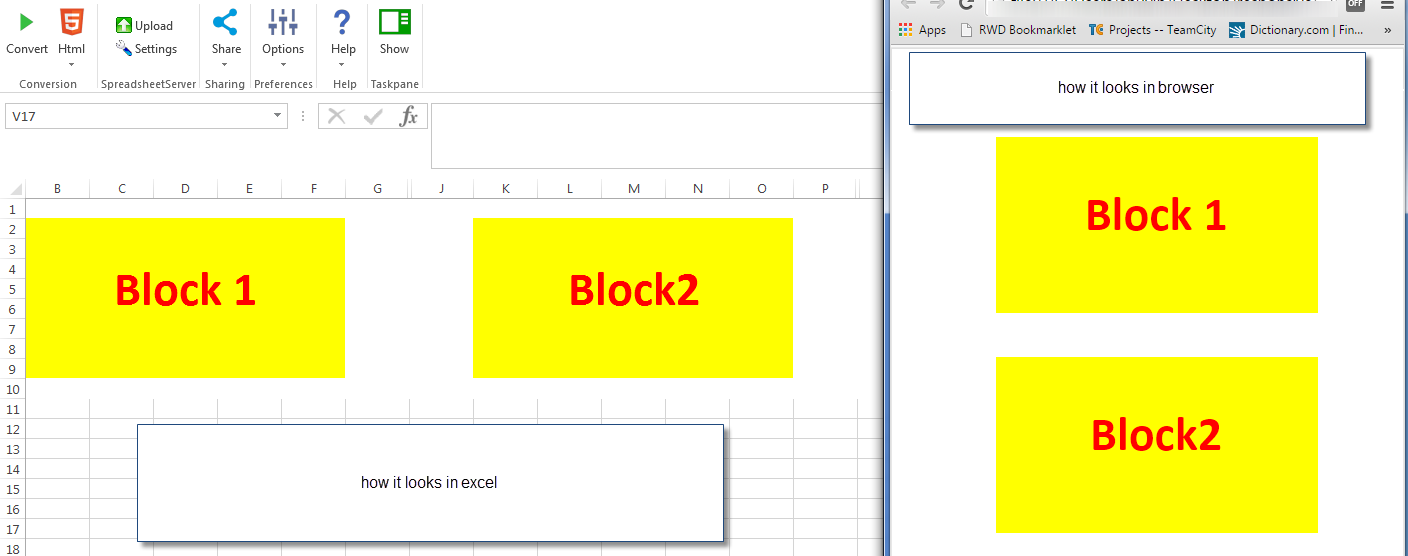
To verify the results in your phone or tablet, use Instant Testing.
Test an example of responsive design in your mobile device
Learn how to edit or delete responsive blocks
Before you create your first responsive spreadsheet, we suggest you read our best practices for responsive blocks to avoid the most common mistakes.
Help: Create a theme with Theme Designer 
Theme Designer 
Create your own theme to make your web calculators look better and have more in common.
Theme Designer is an add-on to SpreadsheetConverter that allows you to set the web page colors you couldn’t set before, e.g. for the page background, for charts and tabs, and for widgets and toolbars. Create your own visual theme and apply it to your web calculators to match your company’s corporate profile – or your personal taste.
The Theme Designer is a free web-based interface where you can create custom themes at http://themedesigner.spreadsheetconverter.com/.
Once you’ve designed a theme, you can download it as a file and use it with your web calculators. Using the ThemePreview toolbar, you can switch between themes directly in the web browser to determine which is best for your calculator. To become permanent, the selected theme must be applied to the spreadsheet before it is converted to a web page.
This help page describes how you can use the Theme Designer to customize the webpages created by SpreadsheetConverter.
Overview 
SpreadsheetConverter converts Excel spreadsheets to live web pages . Most of the formatting of the spreadsheet is preserved, e.g. the text and cell colors, lines and fill patterns that you apply with Excel are also used in the converted web page. Read more about how to format the web page from Excel.
However, Excel does not permit you to set all the properties of the converted page, e.g. the color for the web page background, for charts, tabs, or widgets. We created the Theme Designer tool to give you control over also these properties and to re-use the resulting visual design as a “theme” for more than one calculator.
The finished theme is provided as a Cascading Style Sheets (CSS) file that you download and import into SpreadsheetConverter. The next time you convert a spreadsheet, you can apply the new theme to the converted web page. The theme’s stylesheet contains additional visual properties that are applied when the calculating web page is opened in a web browser.
The ThemeDesigner panels 
The Categories panel 
The Categories panel on the left side of Theme Designer lets you select what part of the web page you want to customize.
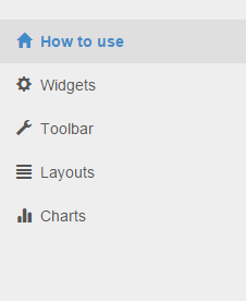
By selecting Widgets, you can edit the brand color of the widgets. On the Toolbar page, you can customize the SpreadsheetConverter toolbar’s color and the color of the buttons. Layouts allow you to modify the colors for sheet tabs and sliding panels. The Charts page allows you to tailor the visual appearance of the charts in your calculator.
The Properties panel 
The Properties panel is in the center of the Theme Designer page. This is where you set the visual attributes for the currently selected category.
For each category, there are different properties you can change. You set each color using a color picker. Click the color picker and select a color, or type the exact Hex color code into the textbox.
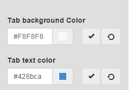
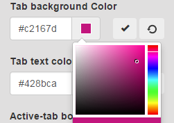
For each color, click the Apply button to the right of the color picker to apply the changes. To return to the initial default value, press the Reset button.
The Preview panel 
The Preview panel is the rightmost panel in Theme Designer. It lets you view the result of your modifications before you apply the theme to a spreadsheet. Whenever you change a visual property, the preview panel reflects the change.
In the below example we typed the Hex color code #42804f into the Toolbar color picker and clicked on the Apply button. As you can see, the Preview panel lets you examine the result.
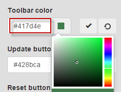

Color spaces and corporate identity 
Both Excel and Theme Designer are built for the RGB color space that is mainly used for display screens. With RGB, the color 0 (zero) is black, as in a dark pixel on the screen. When you work with computer printers, you typically use the CMYK color space. With CMYK, the color 0 is white, as in printing nothing on white stationery. The third common color space is PMS, where the Pantone system is used to select the colors for a printing press.
Using the same colors as in Excel 
Excel uses the RGB color space. If your spreadsheet uses a color that you also wish to use for your theme, simply read the values for red, green, and blue from the Excel color picker.
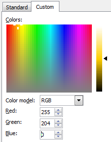
Convert the decimal numbers for Red, Green and Blue to hexadecimal codes with one of the many web tools for this purpose.
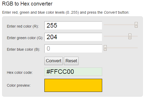
Enter the hexadecimal color code into the Theme Designer color picker.
Using the same colors as in your website 
If you wish to create a theme with the same colors as the rest of your website, you can obtain the proper Hex codes from the stylesheets used for the web site. As an example, if you find that your website uses the color #FFCC00 a lot, you can use the same color for your web calculators by applying it Excel or Theme Designer.
Using the same colors as in your company logo 
If you want to use corporate colors like the colors in your company logo, you may save a lot of time by asking your PR department for the Pantone (PMS) codes that were used. There are tools on the web that help you convert Pantone colors to RGB colors. There are also web tools to help you match a color in an uploaded image.
Applying a theme to a calculator 
When you have set all the colors you require, you download the theme as a stylesheet and import it into SpreadsheetConverter in your PC. You can then apply the theme to any calculator during conversion. Let’s continue with how to download and apply a theme to a calculator.
Learn more 
Some of our tutorials partly focus on themes:
Help: Use both theme and Excel formatting 
Working with layout 
Learn how to format your calculator from Excel and from a theme at the same time.
Theme Designer is a powerful tool that helps you customize parts of the spreadsheet. However, the theme only controls the layout that is not set from inside Excel. This tutorial shows you how the Excel settings for the cells in a form blend with the overall layout settings in the theme.
Example spreadsheet 
Here’s a simple calculator to convert time from one time zone to another – we called it the Global Meeting Planner. You set your time zone and the time zone for the person you want to meet. Using the slider you can scroll through the possible times during the day, trying to find the best time for the meeting. The example calculator has some formatting assigned by the theme, and some coming from the spreadsheet.
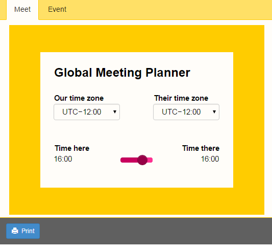
Plain spreadsheet 
To create the example, we started with a plain spreadsheet. You can download the plain spreadsheet here. This is what the spreadsheet looks like without formatting and theme.
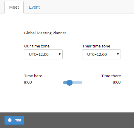
Formatted spreadsheet 
If you just want to use a different color for the text in a cell or change a cell’s background color, use the Format Cells command in Excel before you convert the spreadsheet to a web page.
Now, let’s add some formatting in Excel. Let’s make the font bold and bigger. Let’s fill the surrounding cells with yellow color. Read more about how to format the web page from Excel. You can download the formatted spreadsheet here.
This is what the spreadsheet looks like when we’ve added the formatting in Excel. As you can see, from Excel we cannot format the tab row at the top of the screen – it’s not even part of the spreadsheet. We cannot assign a color to the slider that was added by SpreadsheetConverter, or to any other widget. All this must be done by the theme.
Theme 
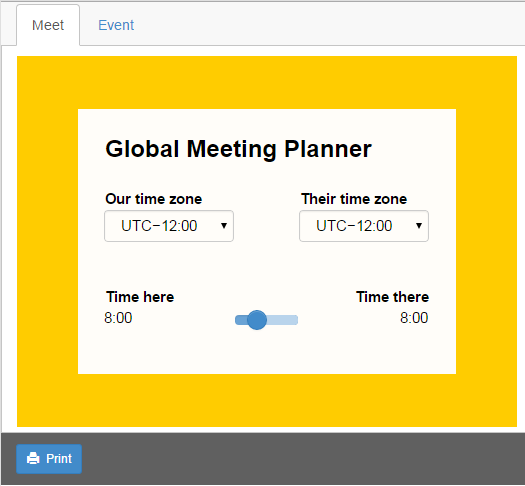
In order to style the rest i.e. tab row and the slider, you need to create a new theme from Theme Designer and use this theme for the spreadsheet.
Inside Theme Designer, click on the Layouts category, then enter the following color values:
- Tab background color box: #ffe066
- Tab text color: #262213
- Active-tab background: #fffdf9
- Active-tab text color: #262213
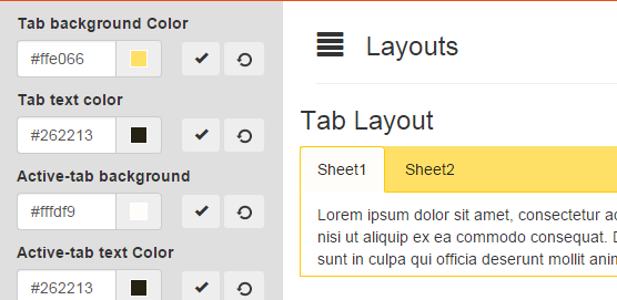
Select the Widgets category, then enter #960046 as the Brand color.

Now, download the theme and apply it to the spreadsheet from the Workbook tab. For your convenience, the theme file can be downloaded here too.
Final Result 
Here is the final calculator, with the correct theme applied. As you can see, the tab row is now adapted to the color scheme, as well as the slider.
This shows that much of the formatting needs to be done in Excel, and that a theme can be used to format the rest.
Now, try for yourself! Try adapting the bottom toolbar and the Print button to the colors of the theme.
Conclusion 
With SpreadsheetConverter you can deliver beautiful calculation and visualization tools to an unlimited number of end users from one common central location. You don’t have to distribute files that eventually become outdated. Your end users don’t even need a license for Excel.
Import an Excel spreadsheet in your blog or website 
Converting spreadsheets to web format makes it very easy to import them into your blog or website. Here are tutorials on how to do this in various popular environments:
- Import Excel spreadsheets and charts in Blogger
- Import Excel spreadsheets and charts in Drupal
- Import Excel spreadsheets and charts in Google Sites
- Import Excel spreadsheets and charts in Joomla
- Import Excel spreadsheets and charts in Squarespace
- Import Excel spreadsheets and charts in Typepad
- Import Excel spreadsheets and charts in Weebly
- Import Excel spreadsheets and charts in Wix
- Import Excel spreadsheets and charts in WordPress with the plugin
- Import Excel spreadsheets and charts in WordPress without the plugin
- Import Excel spreadsheets and charts in any blog or website
Help: Design the web page for ALL your visitors 
Design for all your visitors 
You should design your calculators and forms to work well around the world. It’s easy to forget that many people will view your page on their phones.
Many of the people that will use your form or calculator will be using it on a phone, probably in portrait mode. If you design and test only on your widescreen laptop, you will lose many visitors when they get fed up from scrolling horizontally through your unnecessarily wide layout.
With a global audience, you have to live with a lot of different measurement units, number formats and date/time formats.
To help you design the web page for all your visitors, we created this short checklist.
Design for mobile users 
Always design your web pagesto work well also on mobile displays. Use only one- or two-column layouts. Put the caption on top of each field, not to the left of it. Use placeholder text in each field to make it clear what information you expect in the field.
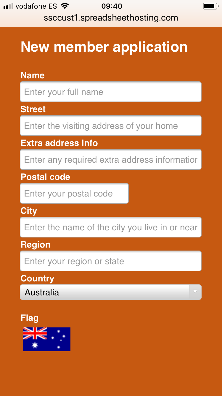
Design vertically 
Arrange the sections of the calculator or form below each other, or on different tabs. Don’t put new things to the right of old things, put them below.
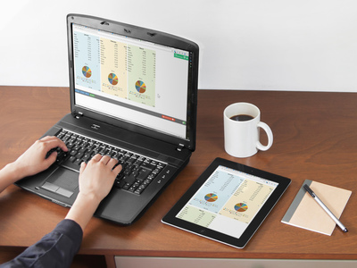
For wider examples, you must use responsive design to make the example fit also narrow screens. In the example below, responsive blocks in the spreadsheet allow three columns on the laptop, two on the tablet and one on the phone.

Don’t use tables, use charts or lists 
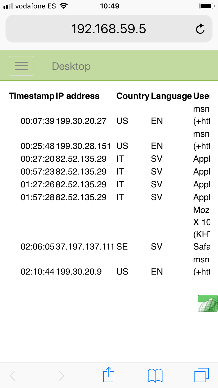
As a desktop user, you may love to analyze data in wide tables with countless columns. This doesn’t work well on phones. You have many options:
- Visualize your data with a chart instead, or show just the subtotals from the main table.
- Move the table to a separate worksheet. Link to it from the main page and open it in a separate window – for enthusiasts only.
- Organize the data vertically, as a list. See the example below how easy it is to make the table easier to read by transposing the columns into rows. It may look boring, but it’s at least much easier to scroll that way.
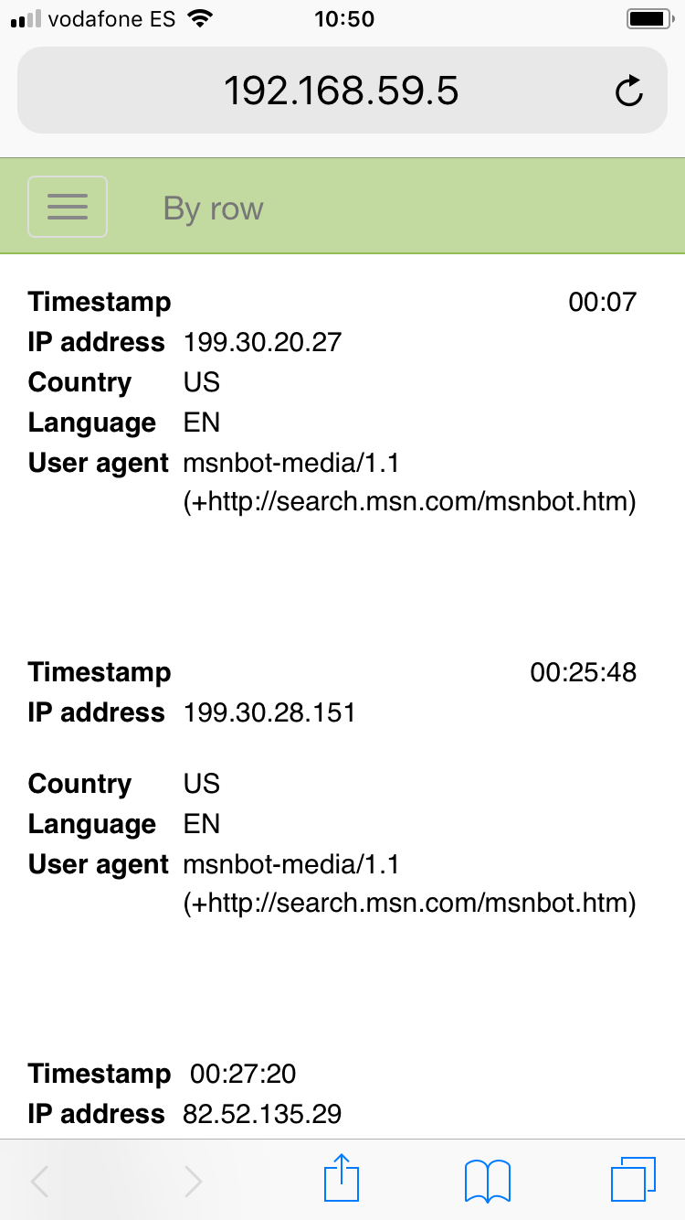
Test everything on your own phone 
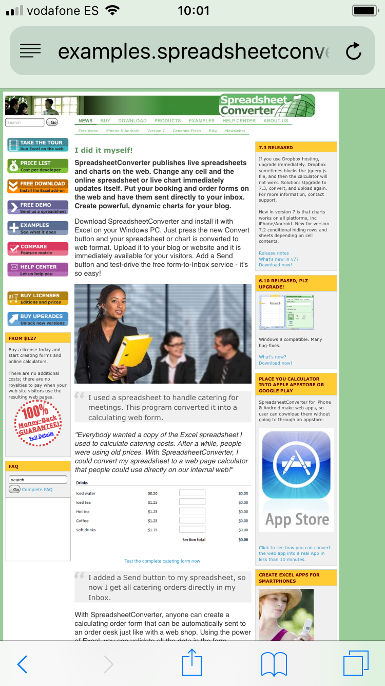
Test every form and calculator also on your own phone, to verify that it looks OK also for mobile users. Which would you rather use on your phone, the old, non-responsive website to the left or the one with responsive design to the right?

Avoid regional differences 
Assume your form or calculator will be used by an international audience.
- People over the world use many different date formats, so avoid using dates in text format if you can. Use a calendar widget to set dates, or separate dropdowns for the year, month and day.
- Avoid using a 12-hour clock with AM/PM notation. With an international audience, you get fewer mistakes with a 24-hour clock.
- Avoid using currency symbols like $ or £. You want your calculator to work also for visitors that use a different currency.
- The natural order of address fields varies between countries. The street number may be before or after the street name, and the postal code can go either before and after the city name.
- Five countries in the world require a region as part of an address: Australia, Brazil, Canada, Great Britain and the USA. In most other countries, there is no region in the address and therefore you must not make the region field mandatory.
- Most countries in the world use decimal comma. You can still use a decimal point, of course, but you should be aware of the issue.
- Most countries use metric units, but some use US customary units like inches, ounces and gallons. Consider offering your users a choice between the two.

Use colors that work for everybody 
Use only colors that are as far away from each other as possible, using colors that are unambiguous also to colorblind persons. It’s easy to work with this helpful table from https://jfly.uni-koeln.de/color/#pallet.
Help: Edit and delete Responsive blocks 
Edit a responsive block 
To update the definition of a responsive block, do as follows:
- Open the Responsive blocks widget from the ribbon.
- Scroll down to the Blocks in the current sheet and click on the name of the block in the list (you cannot select a block with the visualizer).
- Change the range, name and the screen size percentage as required.
- Verify the new layout for phone and tablet in the Preview section.
- Press the Update button to save the new settings.
Delete a responsive block 
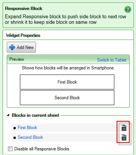

Normally, you shouldn’t delete responsive blocks unless you intend to expand an adjacent block to also cover the cells that were previously part of the deleted block. All active cell areas must be part of a responsive block, so if you delete a responsive block you must always change the definition of another block to cover the affected cells.
To delete a responsive block, just click the “waste-bin” button for the responsive block. Please note that there is no undo for this.
Disable all responsive blocks 
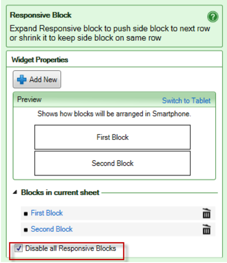

If you have created responsive blocks for a web page, you may still want to go back to the old non-responsive design without losing the responsive block definitions you’ve made. The Disable all Responsive Blocks check-box allows you to generate the web page without a responsive design. Uncheck the check-box to enable responsive design again using the previously saved definitions.
Google Map 
Google Map 
Use the Google Map widget to insert a dynamic map into your form or calculator. You can control what the map is showing from inside the spreadsheet.
The Google Map widget lets you use a map in a web app created from a spreadsheet. You can have the spreadsheet control what area the map shows, and insert pins on specific, named locations.
Google Maps is not an entirely free service. You need a Google account with billing enabled, using a valid credit card that has not expired. Using this account, you request an API key that you use whenever you show maps on your website. The API key is used to pay Google for the map impressions that exceed your company’s free monthly quota. Registering for an API key is free and uncomplicated, but your API key may be stolen if you implement it incorrectly, which may lead to unexpected charges to the credit card you use with Google. If you don’t already have an API key, you must request one from Google.
For this help page we created this example web page: Store-finder web page
from this Excel spreadsheet: Store-finder source spreadsheet
Instructions on using the Google Map widget 
Insert the widget into the right cell 
In the spreadsheet, select the cell where you want the upper left-hand corner of the map. Select the Google Map widget on the Widget tab of the task pane to insert the Google Map widget in this cell. Using the corners and sides of the Google map object, drag it to the required size.
The image shown in the Excel spreadsheet is just a static placeholder and will not reflect the changes you make in the widget’s settings. It is not until you convert the spreadsheet to a web page and load it into a web browser that the actual map appears according to your settings.
Set the basic options 
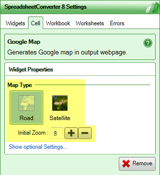
Select the Map Type. A Road map is schematic, a Satellite map is assembled from photos taken from a satellite.
Set the Initial Zoom. This controls how much of the world that is initially shown on the map. To give you an idea of what number to use, you see most of the world at zoom level 3, and the entire USA at zoom level 5. A major city like London fits in a zoom level around 10. A borough like Manhattan or Hollywood is suitable for a zoom level of 15. At a zoom level of 20, small animals like cats and dogs are clearly visible on the Satellite map.
Set the default map location 
Click on the link for Show Optional Settings…
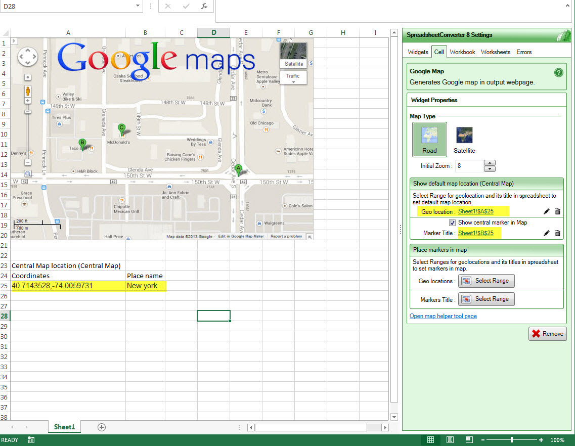
In the Optional settings, you can define what location you want in the exact center of the map. The widget gets these geographical coordinates from a cell in the spreadsheet.
For Geo location, select the cell in the spreadsheet that contains the geographical coordinates for the map center. To determine the coordinates you can use our free map helper tool, see below. You can also use a reasonably exact name that Google understands, e.g. “Alexanderplatz, Berlin, Germany”.
If you want a marker at the center position, tick Show central marker in Map.
For Marker Title, select the cell that contains the title for the map center marker.
Place markers in the map 
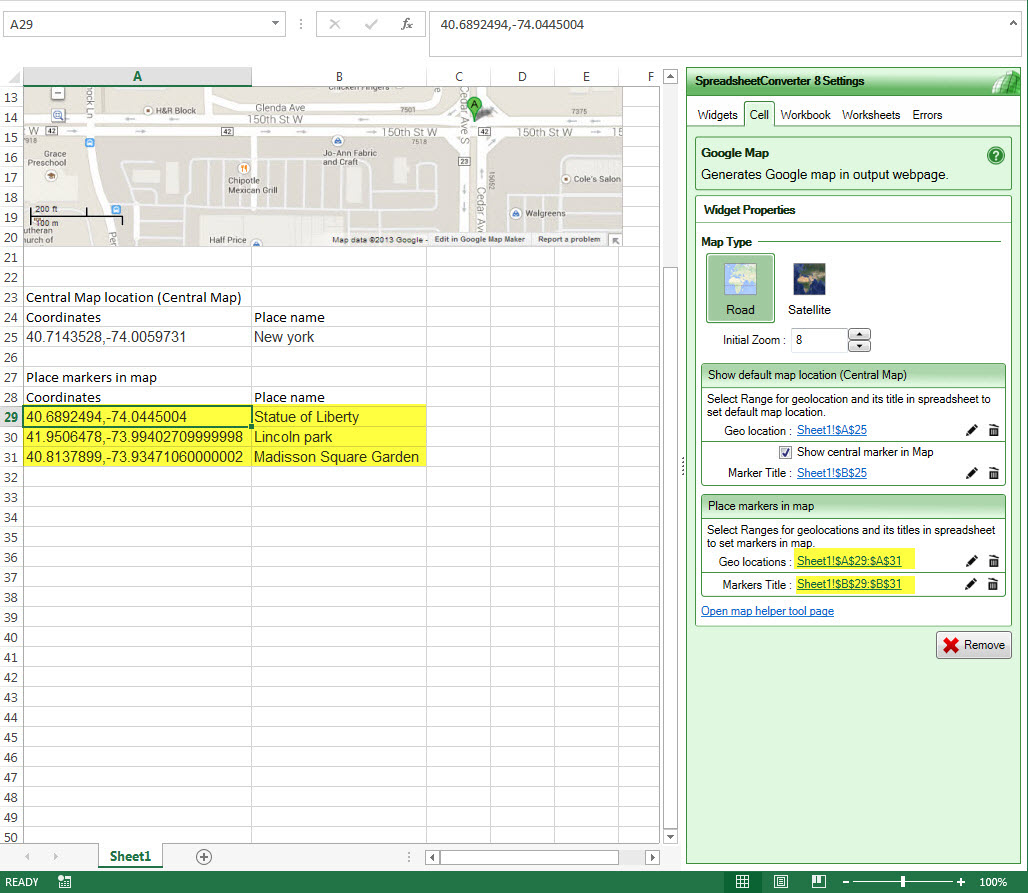
In the Place markers in map section, you can place one or more additional markers on your map with descriptive titles. The widget gets this information from a cell area in the spreadsheet. Just create a list of the location and title for each marker, or copy the Table of markers from the map helper tool (see below) to the spreadsheet.
For Geo locations, select the cell area that contains the coordinates for all locations where you want to place a marker. To determine the coordinates you can use our free map helper tool, see below. The location for each marker can also be specified with a reasonably accurate location name that Google understands, e.g. “Princess Gardens, Toronto, Canada”.
For Markers Title, select the cell area that contains the title for each marker.
Provide the Google API Key 
Before you can use the Google Map widget, you must specify your API key on the Workbook tab. For version 1-8, please read the Known issues below.
Convert the spreadsheet 
Save the spreadsheet and convert it. After the conversion, the converted web page will open in one or more of your browsers, and you can see the result of your settings.
If your Google map does not appear, and you get a text saying Oops! Something went wrong or similar, there may be a problem with your Google Maps API key.
The Map Helper Tool 
Our free Map Helper Tool lets you create a preview of a map you want to show in your spreadsheet. The Map Helper Tool is a simple web app that lets you tailor the zoom level, find the appropriate center location for the map and place the markers you need on the map.
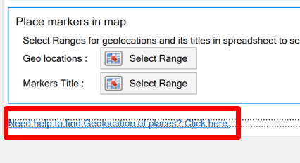
Click on the link to the Map Helper Tool at the bottom of the Optional settings for the Google Map widget to open the tool in your web browser.
Use the text field at the top to search and position the map approximately where you want it.
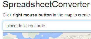
As you can see, the tool automatically centers the map on the requested location and inserts a marker. If necessary, drag the marker to the exact location. If you intend to place a marker in the center of the map, you should also enter a title for it.
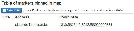
All marker coordinates are saved automatically in the Table of markers below the map, so you don’t have to save anything manually. However, if you remove the selected marker by clicking Remove me, you may want to save its coordinates first as this will also remove it from the Table of markers.
You can add additional markers manually by right-clicking anywhere on the map. You should enter a title for each marker.
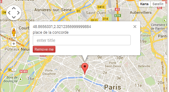
All locations you search for and all markers you add manually are saved in a Table of markers below the map. You should enter a title for each row in the table. When you have marked all locations, you can select the entire list and copy it over to your spreadsheet with Ctrl-C.
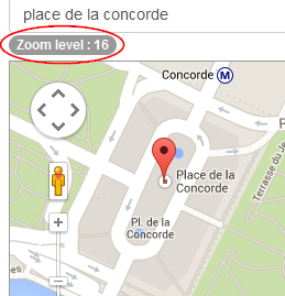
Use the zoom selector on the left side of the map to find the appropriate zoom level for your map. The selected zoom level is shown above the map. Just copy this number to the Initial Zoom setting for your Google Map widget.
Known issues 
Edit the conversion result and add your unique Google API key 
If you are using version 1-8 of SpreadsheetConverter, you need to manually add the API key to the converted web page after you have converted the spreadsheet. Otherwise, your map may look like this:
Add the add-in to Excel manually 
Help: Add to Excel manually 
These are the instructions to add SpreadsheetConverter manually to Excel
Add the add-in to Excel manually 
Follow these instructions to add the add-in manually to Excel, if all other installation methods fail.
In some situations, SpreadsheetConverter cannot be installed automatically. One common reason is that you have installed Excel and the rest of Office from Microsoft Store.
The most obvious symptom is that the menu ribbon is not visible in Excel, and that the add-in is not on the COM Add-ins list.
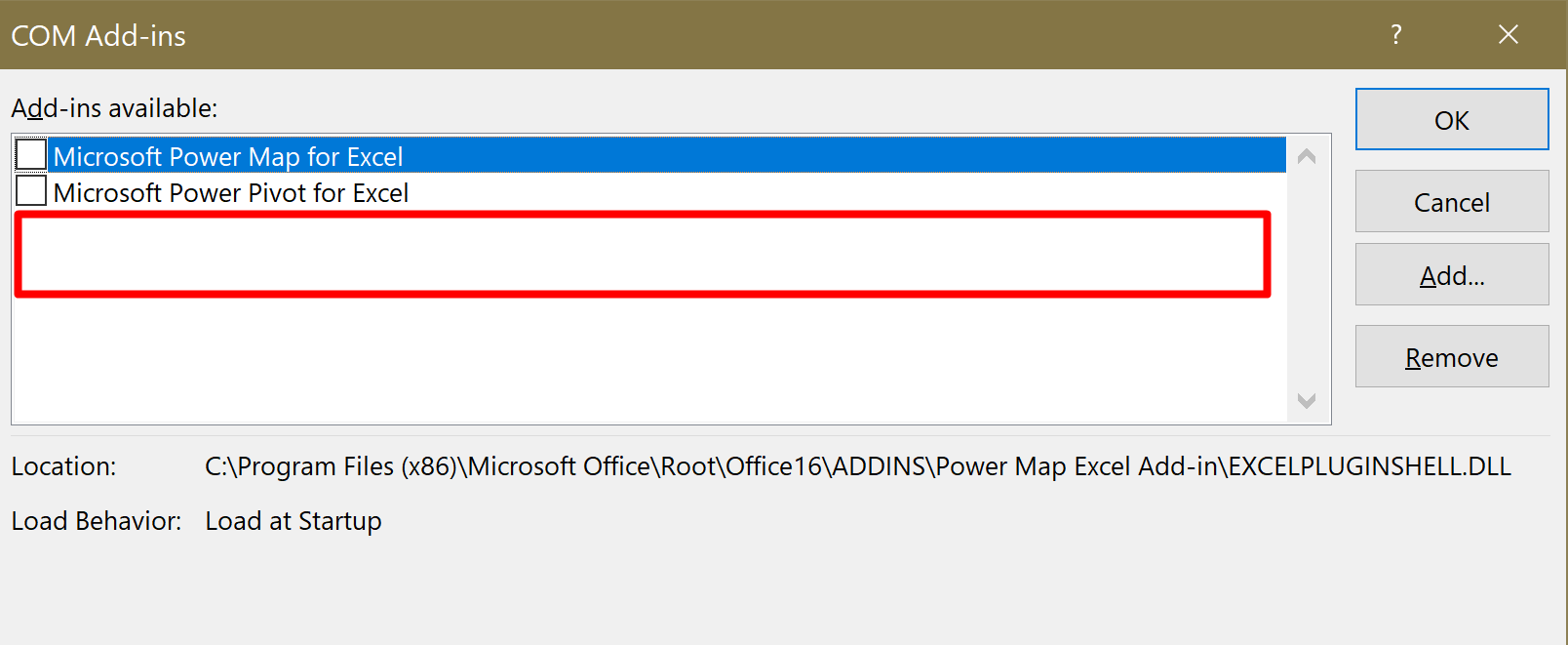
Follow the simple instructions below to manually add the add-in to Excel.
Determine the Office version 
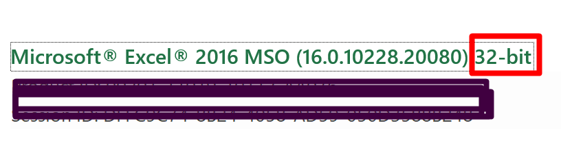
There are 32- and 64-bit versions of Excel. You are probably using a 64-bit version of Windows, but that doesn’t necessarily mean you are using a 64-bit version of Office. For this operation, we absolutely need to know which version you have. Follow these steps to determine which version you are using:
Start Excel and open a new, blank workbook.
Click File > Account > About Excel.
Locate the version number and note if your Excel is 32- or 64-bit.
Add the add-in to Excel 
In Excel, go to File > Options.
Select the Add-ins tab.
Locate the Manage drop-down list at the bottom of the Excel Options window.
Select COM Add-ins.
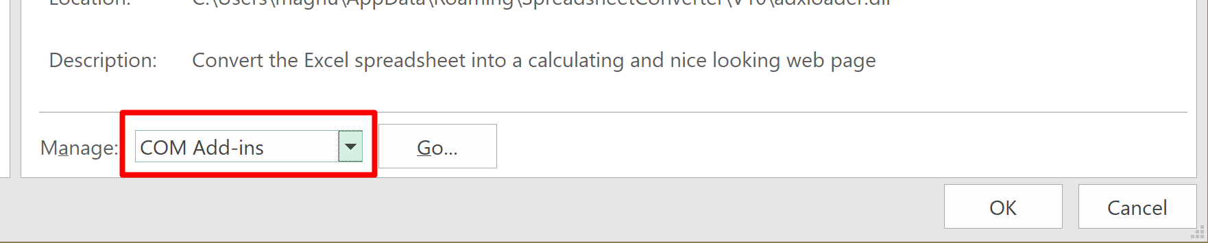
Click Go.
If SpreadsheetConverter is not in the list of COM Add-ins, click Add.
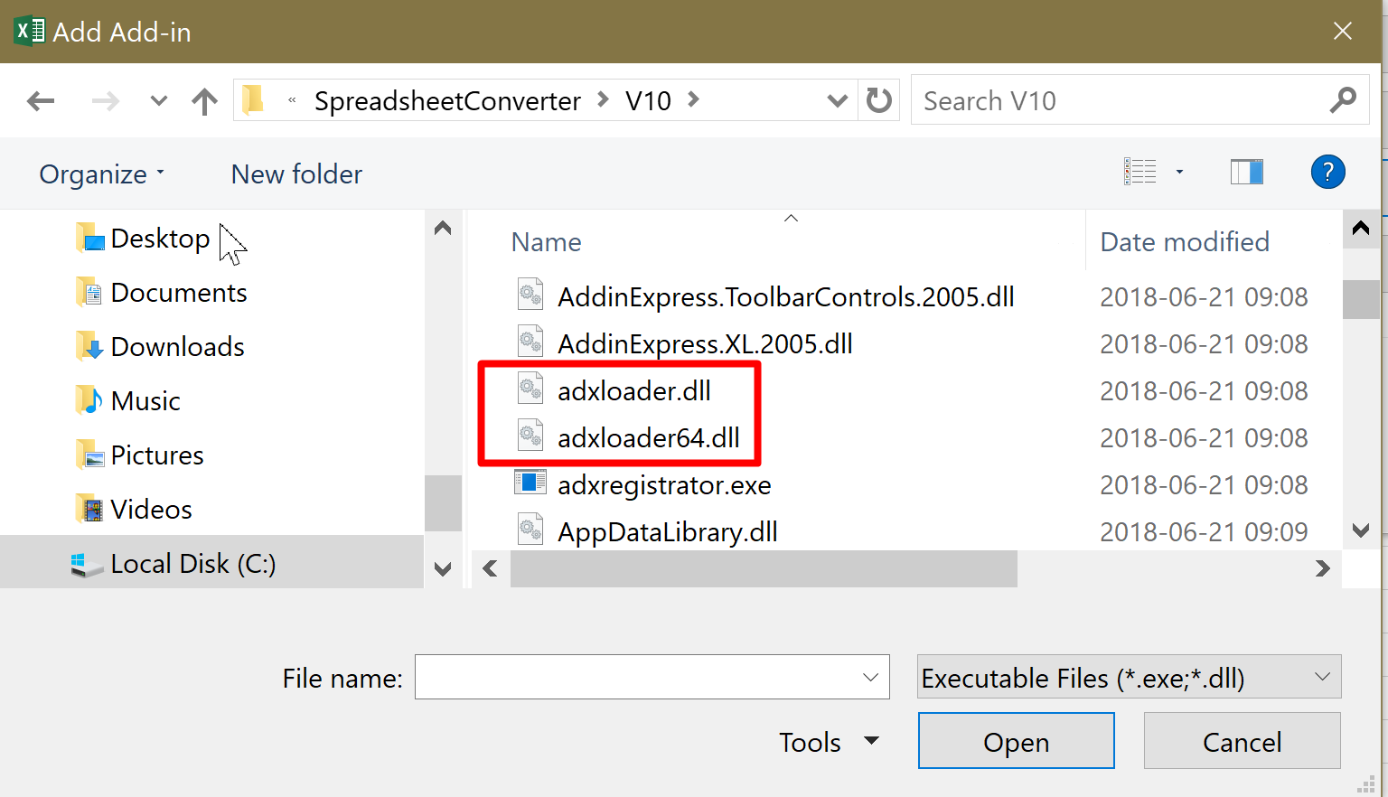
Navigate the add-in’s installation folder. By default, this is Users > [Name] > AppData > Roaming > SpreadsheetConverter > version. You may have to check View > Show hidden files… in the Control panel’s Folder options to make the AppData folder visible.
- If you are running 32-bit Excel, select the file adxloader.dll.
- If you are running 64-bit Excel, select the file adxloader64.dll.
Click OK.
The add-in should now be installed in Excel and appear in the list of COM add-ins.
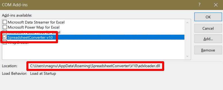
Ensure that the checkbox is ticked, press OK and restart Excel if necessary to make the SpreadsheetConverter ribbon menu appear in Excel.
Verify that the add-in is correctly installed 
You should now see the SpreadsheetConverter add-in in the Excel menu.

If you still have problems, don’t hesitate to contact our Help Desk.
The Barcode widget 
The Barcode widget 
The Barcode widget lets you generate a scannable barcode directly on the web page. The code can contain static information or information dynamically obtained by calculations or lookup operations in the spreadsheet.

Barcodes are one-dimensional, linear images containing information that typically identifies the object that carries the barcode. Most items in today’s shopping malls are marked with barcodes that are used to look up the price for each scanned item and add it to the total.
Barcodes are also used for tracking purposes. Many trackable object like vehicles, containers, pallets, bags and parcels carry a barcode that identifies the object and makes it easy to track it during transportation.
In your office, there may be barcodes mounted discreetly on the walls. If a passing guard scans these barcodes, it is easy to track the areas of the building that have been surveilled.
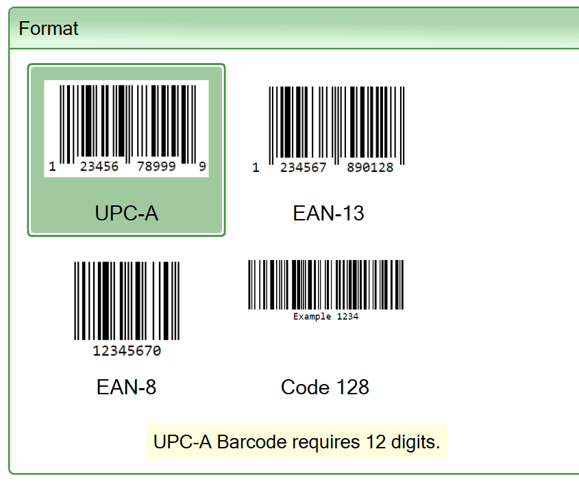
Barcodes can be scanned directly off the screen or printed on labels. In this first release, we support the following barcode formats:
- UPC-A – retail product numbers.
- EAN-13 – retail product numbers, succeding UPC-A.
- EAN-8 – 8-digit EAN version.
- Code 128 – used extensively in the shipping and packaging industries as an identification of containers and pallets.
Adding a barcode to your web page 
The barcode widget uses two cells in the spreadsheet, one for the source data and one for the generated barcode. To create the widget, select the cell where you want the upper left-hand corner of the barcode. Open the task pane and select the Widgets tab. Scroll down to the Barcode widget. Click on the icon to insert the widget into the selected cell.
The barcode format 
The widget can generate the barcode in different formats. Select the format you want in the Format section of the widget properties.
The source data cell 
The content of the barcode will be taken from one of the cells in the spreadsheet. The source data cell can contain a static value or calculate the barcode contents with a formula. Static and calculated values can be concatenated.
To select the source data cell, click on the Select a cell button, click on the source data cell and then click OK. You can also type a cell reference into the text box and press OK.

The barcode width and height 
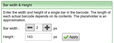
Set the width of each bar in the barcode in pixels. The wider the bars are, the longer the barcode will get. If the barcode is too long it may not fit the screen, or be difficult to scan.
Set the height of the barcode in pixels. If the barcode isn’t high enough, it may be difficult to scan.
The barcode placeholder 
When you insert a barcode widget in a cell, a placeholder appears in the same format as the barcode will have in the converted web page. Each actual barcode is generated starting at the upper left-hand corner of the placeholder and becomes as long as required by the data.
When you edit the spreadsheet in Excel, the placeholder will not reflect the current value of the source cell. In the example below, the source data is in A1, but as you can see the barcode placeholder is unaffected. Like most widgets, the barcode widgets are live in the converted web page, but not in Excel.
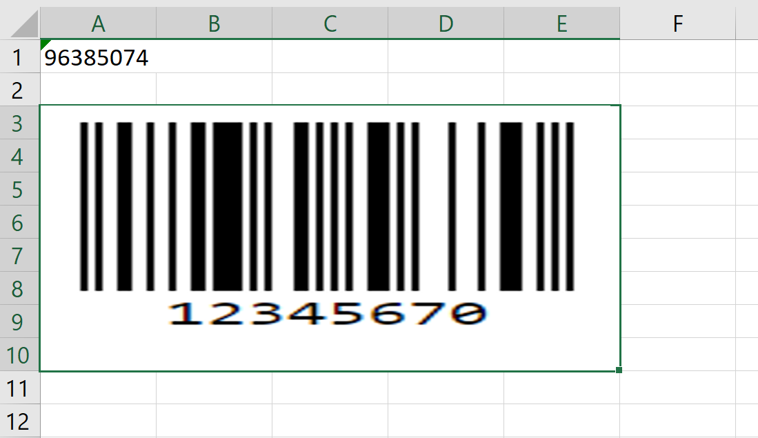
When you work with widgets that use placeholders, you will often get a better result if you merge all the cells behind the placeholder. This enables the converter to better determine the size of the widget as it will appear on the web page. In the example above, we have merged cells A3:E10 to make room for the widget.
The size of the placeholder in Excel is an approximation based on your settings for the barcode widget. The best way to change the size of the placeholder is to edit the settings. If you don’t think the placeholder has the correct size, you can drag the corners of the placeholder to adjust it. The size of the placeholder has no effect on the actual barcode on the web page.
Checksums and data validation 
Almost all barcodes contain extra information that helps detect scanning errors. Usually, there is a checksum that must validate against the rest of the field contents. This information is not part of the actual product, account or ticket number, which may contain its own checksum.
The checksum is only relevant during data entry, i.e. when the barcode is scanned or the corresponding numbers are manually typed into an input field. When saving the scanned product number you typically don’t save the checksum with it since it isn’t a part of the number.
You need to validate the data used with a barcode 
The barcode widget does not validate any part of the code you provide. If the source data for a barcode is typed manually into a form, you must validate it before you use it to generate a barcode.
- Numeric barcodes must contain digits only. You cannot allow blanks, commas, periods or any other character to be used as source data for a numeric barcode.
- Numeric barcodes consist of strings of digits. To preserve the contents of such numeric strings, you must carefully ensure that you handle them as text strings throughout the process. Otherwise Excel may treat the code as a number, which usually means that it right-adjusts the number in the field and trims any leading zeros. When displaying the code as a number, Excel may impose decimal or thousand separators, and for a large number even switch to floating point notation. If your 12-digit EAN product code looks like 1,23456E+11 in Excel, your numeric product identification string is being treated like a number and may generate incorrect barcodes. Start by giving the input cell a Text display format in Excel.
- You must verify that the source data has the expected length, e.g. 11 or 12 for a UPC barcode.
- If a product number is composed of known parts, e.g. it has a manufacturer code and a product code, you can verify these separately with IF clauses or lookup operations in the spreadsheet.
- In certain applications, two or more barcodes are used in conjunction. e.g. for a book’s ISBN or on the waybill for a courier or postal consignment. You must ensure that the contents of the different barcodes match.
We will auto-correct some errors in your data 
If the source data you assign to a barcode is incorrect, the barcode widget may generate a different number than you assign to it. We have no proper way to signal source data errors back to the form. Automatically correcting the data provided by your spreadsheet simplifies the coding of the spreadsheet and reduces errors.
- When you assign a number to a barcode that has a checksum, the barcode widget enforces the correct checksum automatically. This simplifies your spreadsheet design without reducing data quality. We allow you to provide all 13 digits for an EAN-13 barcode, but the widget will only use the first 12 digits and end the barcode with the correct checksum digit. If you provide source data with an incorrect checksum like 6543211234561 for an EAN-13 barcode, the barcode will still be generated as 6543211234566 with the correct checksum digit at the end.
Known Issues 
- The Barcode widget is only supported in the Professional edition of SpreadsheetConverter. Upgrade to the Professional edition to use more charts, extra powerful widgets, more Excel functions and many other advanced features.
Customize and translate text 
Customize and translate text 
Follow these instructions to customize and translate the various standard texts in online spreadsheets and web forms generated by SpreadsheetConverter.
Although the SpreadsheetConverter program itself is currently only available in English, the conversion process and the conversion results can be used with any language. For an overview of the translation features, please begin by reading the Translation Overview.
The text management features in SpreadsheetConverter also allow English-language users to adapt all application-generated texts to their individual needs – add a business term to the input prompts, the help desk’s phone number to critical error messages or use local terminology like Process instead of Submit in button labels.
Customize text 
The Customize text settings in the Options > User Settings window control most of the built-in language support.
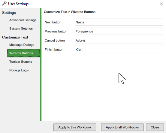
- Message Dialogs
Use your own vocabulary when telling website users that a form is missing certain mandatory input fields. Customize or translate the information that is provided when an electronic form is submitted, or when Offline Submit kicks in because the user is offline when trying to submit a form. - Wizard buttons
Customize the Next and Previous buttons found in a step-by-step “wizard” dialog, and of course the Cancel and Finish buttons. - Toolbar buttons
Change the text used for Submit, Print and the other standard buttons on the toolbar: Print All, Reset and Update. - Node.js Secure Login
When a web calculator or electronic form should be available for authenticated users only, you can create a login page when converting for Node.js. All the text on this page can be changed any way you like it.
Data Validation 
Data Validation 
Instructions for how you use Excel’s data validation features in online spreadsheets.
Data Validation 
Follow these instructions to use Excel’s data validation features in online spreadsheets and web forms generated by SpreadsheetConverter.
Excel provides a number of built-in data validation features that makes it easier for you to ensure that electronic forms only contain valid information. SpreadsheetConverter supports most of these rules, and will enforce these rules also in the converted web page.
Using Data Validation in the spreadsheet 
To validate input data in a spreadsheet, Excel allows you define rules for each cell in the Data > Data tools > Data Validation section of the Excel menu. For more information about the Data Validation feature in Excel, please study Excel’s Help pages.
You can assign unique rules for each cell in the spreadsheet. The validation criteria supported by SpreadsheetConverter are:
- Whole number
The value in the cell is an integer. You can limit the allowed range of integer values, e.g. 1-5. - Decimal
The value in the cell is numeric. You can limit the range of numeric values, e.g. 3.1415-3.1416. - List
SpreadsheetConverter converts this to a dropdown menu with static choices. The Source field must contain a static cell range; you cannot use functions like IF, INDEX, INDIRECT, MATCH or OFFSET here. The cells in the designated cell range can only contain static text. If you need to use dynamic text for the choices in a dropdown menu you should use the Dynamic Dropdown widget. - Date
The value in the cell is an Excel serial number; a timestamp. You can limit the allowed range for the date portion of this timestamp. Some examples include conditions like invoice date must be a past date, event date must be a future date, delivery date can’t be on weekends, etc. - Time
The value in the cell is an Excel serial number; a timestamp. You can limit the allowed range for the time portion of this timestamp. - Text length
The number of characters in the cell must conform to these rules, e.g. the cell must contain at least eight characters. - Custom
The value of the cell is evaluated using an Excel formula. The formula can test for almost anything, e.g. that a date refers to a Monday or that there is a number in the cell that is a multiple of 12 or total expenses must be under the budget etc. It can be used to avoid duplicate entries or validate product code or special format too.
Ignore blank setting 
The Ignore blank checkbox skips the validation rules for empty fields. Tick this checkbox for fields that should be validated only if they contain something.
Specifying Error message 
You can specify what message to display if the field contents are invalid. You can do so from the Error Alert tab of the Data Validation dialog box. Enter your message in the Error Message box. The Title box is not supported.
In the Style dropdown, choose the Stop style if you want to prevent the form from being submitted if the field contents are invalid. The error message will be in a red arrow pointing to the invalid field. Choose the Warning style to have the message appear in a yellow arrow or the Information style for the message to appear in a blue arrow. Always tick the check box Show error alert after invalid data is entered.
The Input Message tab is not supported. Add text near the cell if you need to tell users what kind of data they are expected to provide.
Validating an e-mail address 
One of the most common and also most complex data validations is to verify that e-mail addresses are correctly written, e.g. that there is only one @ sign, that there is text on both sides of each period etc. The syntax rules for an e-mail address are far too complex to be handled with Excel Data Validation or Excel formulas.
Instead, use the Text > E-mail widget which is a standard text field with built-in validation of e-mail addresses. The field must either be empty or contain a valid e-mail address. If the e-mail address has an incorrect syntax, or if the field is empty but set as Required, the field is considered in error and the form cannot be submitted. This reduces the risk that you receive forms with missing or incorrect e-mail addresses.
The widget only validates the character string in the field; there is no live or online validation that the provided e-mail address actually exists or that someone reads the e-mails sent to it.
Known issues 
If you are validating a date, and you enter the date directly into the Start Date or End Date fields, you must use the system date format specified in the regional settings control panel. If you would prefer to use a different date format, please place the date in a separate cell on the worksheet and give it any date format you like. Then insert a cell reference in the Start Date or End Date fields, i.e. if you’ve placed the date in cell B10 then type =B10 into the Date Validation window. To hide the date so that it doesn’t appear in the converted web page, use the Utility widget or place the date on any hidden row, column or worksheet.
Dynamic dropdown menu 
Dynamic dropdown menu 
This is the Online Help page for the dynamic dropdown menu widget in SpreadsheetConverter.
Dynamic dropdown menu 
This is the Online Help page for the dynamic dropdown menu widget in SpreadsheetConverter.
The purpose of the Dynamic dropdown widget is to make it easy to create a dropdown menu where the options are controlled from the spreadsheet and can be changed by a formula. If you only need a simple, static list of options, it is usually easier to use the ordinary Dropdown list widget in the Basic widgets category.
Due to the inherent complexity of the Dynamic dropdown widget, it cannot be tested in Excel. You must convert your spreadsheet to a web page to test a Dynamic dropdown menu.
The Dynamic dropdown widget operates in one of two modes, either with a one-dimensional table or a two-dimensional indexed table with lookup.
Generate options from a fixed row or column 
In the one-dimensional mode, you provide a list of options in a cell range in your spreadsheet. The cell range can be either row- or column-oriented, and empty cells are ignored. The widget illustrates this, with a cell range containing three choices in a row.
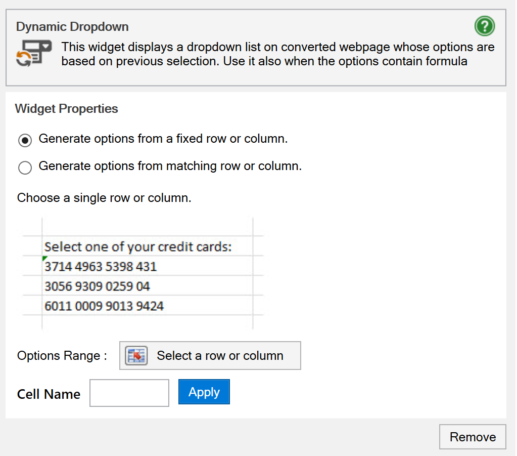
In contrast to the basic dropdown widget, however, this cell range need not contain a static list of choices.
- You can ask a customer to select one of the credit cards that the customer has on file.
- In an order form, you can have a “Quantity” menu for each product contain a dynamically calculated list of accepted ordering quantities, i.e. the number of items in a box, carton or pallet.
- You can create a list of only those account numbers that are eligible for a certain transaction, e.g. checkings or savings accounts.
- You can provide a list of destinations that only include those destinations that fulfill a set of criteria defined elsewhere in the spreadsheet.
Each cell can contain a different formula that assembles, calculates or conditionally selects content for the menu item. Here are a few examples of formulas you can expect to find in a dynamic dropdown:
-
=if(country_name="", city_name, city_name & ", " & country_name)
-
=vlookup(postcode, postcode_to_city_table, 2, FALSE)
-
=if(location_1_available, location_1_name, "")
Make the cell range big enough to accommodate the largest number of choices you will ever need. If you don’t need all choices there’s room for, just leave the redundant cells empty and they will be ignored when the dynamic dropdown is created.
If you want to add a prompt, e.g. Select one of your credit cards on file at the top of the menu, just make it the first choice in the cell range.
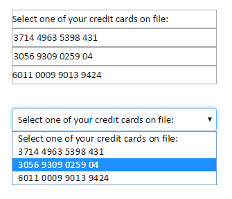
Learn more 
There is an example of a one-dimensional Dynamic Dropdown in the tutorial for the Link Image widget
Generate options from matching row or column 
The two-dimensional mode is best explained with an example. Let’s say we want to show the world’s biggest cities per country. We create a list of countries in a column, and a list of cities in the same row as the corresponding country.
In the table below, the index is located in the first column, in cells A2:A11. For each country, there is a list of cities on the same row. For Japan, the biggest cities are Tokyo, Osaka and Nagoya, in that order.
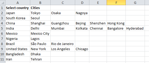
It is very easy to display this index as a country selector, using a one-dimensional dynamic dropdown. Note that we have already placed a user prompt in cell A1 at the top of the list. Just select A1:A11 in the worksheet above as the cell range to provide the choices for the one-dimensional dynamic dropdown.
When the web page is shown in the web browser, the dropdown menu will display the user prompt Select country. In the example, the user has selected India.
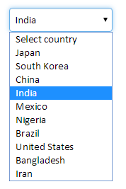
When the user moves on to the second dropdown, its contents are set dynamically, depending on the country selection. For India, the choices are located in cells B5:G5 of the spreadsheet above, and the city dropdown would immediately change to look like this:
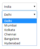
Every time you change the country in the upper dropdown menu, the appropriate cities appear in the lower dropdown menu. This can dramatically increase the speed of data entry, the accuracy and the quality of an electronic form.
Settings for the two-dimensional mode 
In the two-dimensional mode, you provide the cell range for an indexed, two-dimensional table in the Options Range setting.
First column 
Do you want the index in a column, with the options in the cells to the right, as in the country/city example above? We call this the (Index is in the) First Column setting. If the index is longer than the longest list of choices, this may be the easiest layout to work with.
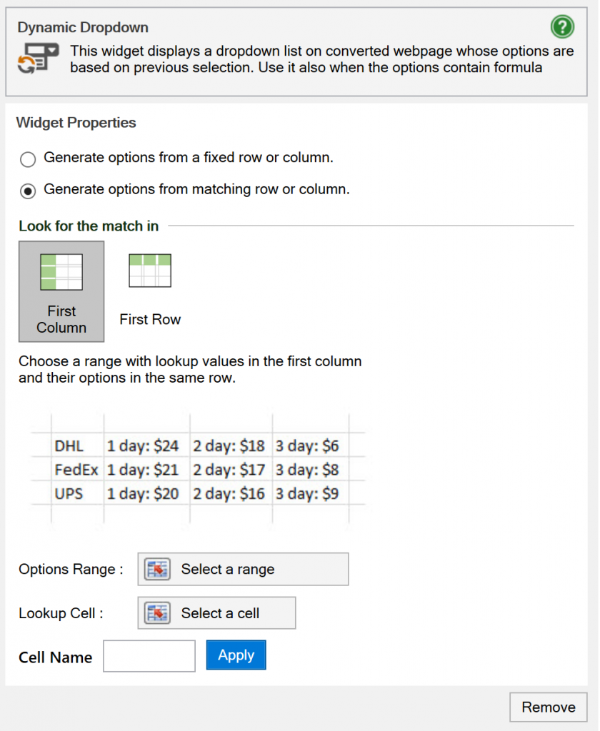
First row 
If the index is short but the number of options can be long, it may be more convenient to use the (Index is in the) First Row setting. In this setting, the top row of the Options Range contains the index, with the menu choices for each key in the cells below it.
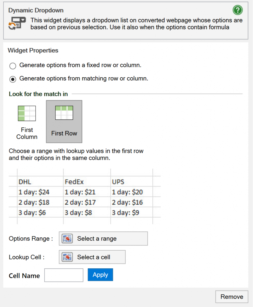
A separate Lookup Cell is matched against the index. In the “major cities” example above, the Lookup Cell is the one-dimensional dropdown used to set the country. It can contain the value Japan. When the Lookup Cell matches a key in the index, the dynamic dropdown menu is populated with all the menu choices for that key. For Japan, those choices are Tokyo, Osaka and Nagoya.
Dynamic Lookup Cell 
You can use many types of widgets for the Lookup Cell, e.g. radio buttons, sliders and even check boxes.
The value for the Lookup Cell doesn’t have to come from a widget, any cell in the spreadsheet can be used for lookup.
- You have a table of sales tax (VAT) per country, and you already know the country from the ship-to address.
- You have a survey where questions are responded to with either Yes/No or the values 1-10. Instead of defining all the dropdowns manually, you use the same options range for all questions in the survey and use a fixed setting per question to select the response type. If you later want to change the options to True/False or 1-5, you only have to change the options range.
Dynamic menu contents 
Dynamic dropdowns take their choices from a cell range in the spreadsheet. You may fill this cell range with any kind of content and change it depending on other cells.
As an example, you may know the origin, destination, dimension and weight for a pending shipment. Using this information, your spreadsheet dynamically assembles a price list from three couriers. All the user has to do is to determine the urgency and pick the best choice.
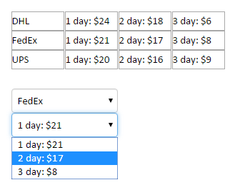
Advanced applications 
Why stop at only two dimensions?`You can use one menu for a country, a second for postal codes per country, and a third for cities per postal code. And a fourth for streets per city! There is no technical limit to the number of levels or “dimensions” in such a menu structure.
You can create all the menu choices in the Options Range using the same programming techniques as we described for the one-dimensional dropdown above.
Known issues 
- If a cell within the options list has a currency format, this number format is not retained when displaying the dropdown. This is a known error and will be corrected in a future version.
The Worksheets tab 
The Worksheets tab 
The Worksheets tab lets you select the worksheets that will be visible on the web page. If your users need to print some of the information in a form or calculator, you may provide a specially formatted print sheet.
The Worksheets tab of the task pane contains a list of all the worksheets in the workbook you are currently editing with Excel. You can hide all the background sheets that you don’t want to be visible in the converted web page. A special worksheet can be used when printing a form.
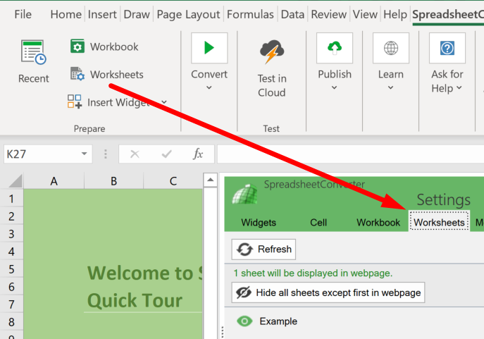
Hide background worksheets in the web page 
When there’s more than one worksheet in your workbook, we automatically hide all but the first during the conversion to a web page. This is because an overwhelming majority of the workbooks with two or more worksheets use only the first worksheets for display – the rest of the worksheets just provide background information for the “front page”.
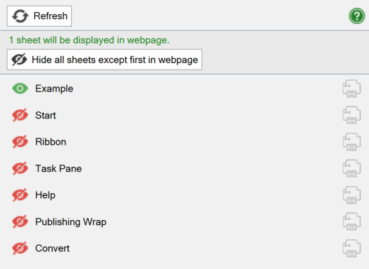
If you want to make more than one worksheet visible in the converted web page, click on the corresponding “eye” symbols in the list so that they turn green before you convert the spreadsheet.
By default, each worksheet appears as a separate tab in the converted web page. SpreadsheetConverter offers various other ways to display multi-section forms and calculators, e.g. as a step-by-step wizard or as sliding panels. Read more about multi-section forms.
If you add a new worksheet to the Excel workbook, it may not be immediately visible in this list, To refresh the list, click on the Refresh button at the top.
Selecting print sheet 
If your users need to print some of the information in a form or calculator, you may provide a specially formatted print sheet that looks better on paper than just a plain print or a screenshot of the browser tab.
You select the print sheet by clicking on the corresponding printer symbol on the Worksheets tab. Only one worksheet can be selected as the print sheet. To unselect the currently selected print sheet, click on the printer symbol again.
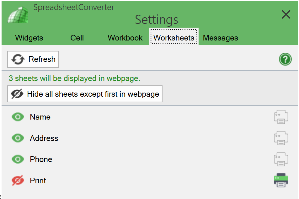
A print sheet is not hidden by default, but if you have created it specifically for printing it’s unlikely that you want the print sheet to be visible in the converted web page. You can hide it by clicking on the eye symbol in the left-hand column until it’s red. During the development of the print sheet, you may want to leave it visible so that the formatted result appears in the Live Preview.
Formatting the web page 
Formatting the web page 
When you convert a spreadsheet to a calculating web page, the formatting is mainly copied from Excel. If your spreadsheet looks good, so will your web page. You can then apply a theme from the Theme Designer.
One of the many strengths of the spreadsheet concept is the easy handling of rows and columns. When creating a spreadsheet in Excel you can tailor the exact appearance of each row and column, including
- row height
- column width
- row/column border lines
- row and column headings
Most of these settings are retained when you convert the spreadsheet to a web page. There are also numerous ways to format individual cells, including
- how to align the content in the cell
- what text fonts to use
- how numbers are displayed
- what colors and patterns to use for text and background
- merging adjacent cells into one
- conditionally format a cell depending on its content
Once again we will do our best to have the converted web page look like the original spreadsheet. If you find that the output of a conversion doesn’t exactly match your intentions, you may first want to go back to the Excel spreadsheet, adjust the formatting and convert the spreadsheet again until it is perfect.
When you’re done with the settings in Excel, have a look at the Theme Designer and see if using a theme can enhance the page further.
Excel defaults to watch out for 
When you create a new spreadsheet with Excel, a large number of default settings are applied. Some of these may be obvious, others may depend on the situation, and a few are downright peculiar, in particular in a web environment.
Regional settings 
Excel uses the regional settings in Windows to determine things like
- The display formats for dates, including the first day of the week
- The display format for times, including whether to use a 12- or 24-hour clock
- The display formats for currency amounts, including separators and the default currency symbol
- The display formats for numbers, including whether to use decimal point or decimal period and how to group digits for high numbers
The converted web page will automatically format dates, times, currency amounts and numeric values according to the regional settings that were in effect during the conversion. If you wish to create a web calculator for a different country or region, or for a global audience, you may want to change the regional settings in Windows before you perform the conversion.
The dreaded ####### 
If a cell is too small for its contents, Excel will truncate or wrap text. For numbers, however, you will get a warning if the contents don’t fit the cell – the entire cell is filled with number signs: #######. This is to avoid showing a partial number that may be misinterpreted as being the complete number.
Before converting a spreadsheet to a web page, ensure that all numeric fields are wide enough to contain all possible values.
Vertical alignment 
By default, Excel has a rather peculiar habit of aligning rows at the bottom. If you insert a Calendar widget you may get the following result:
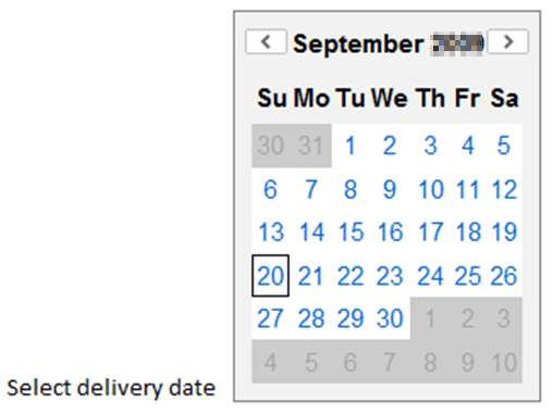
This is because by default, Excel will align the cells at the bottom. Change the vertical alignment from Bottom to Top to make your spreadsheet easier to read:
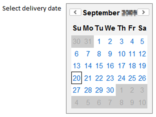
Static content 
A spreadsheet usually has a lot of content that cannot be changed when the spreadsheet is used:
- Formulas
- Field captions
- Instructions
- Hyperlinks
- Copyright notices
- Drawings
- Images and photos
- Locked values, e.g. a credit card fee as a percentage.
There is also often suggested content that can be changed when required.
- Default values, e.g. quantities
SpreadsheetConverter supports all this. Any static content you provide in the spreadsheet will also be present in the converted web page.
One major difference between the spreadsheet and the web page is the locking of the cells. In a spreadsheet, all cells are typically unlocked, which allows you to type a static value into a cell that has a formula. In the web page, all cells are locked by default. Opening cells for input requires special consideration.
Making widgets look good 
Merging adjacent cells 
Widgets use the same row/column layout as the rest of the spreadsheet. Many widgets require more space than the default row height and column width in Excel.
As an example, if you use a dropdown list, a listbox or radio buttons to select a city or state name from a list, you probably want the widget to be wide enough for the longest name in the list. If you don’t, SpreadsheetConverter must either wrap the longer names over more than one line or truncate the names after the allotted width. Neither option really looks good.
If a widget is too big to fit within its cell’s height and width, the corresponding row and/or column may be widened automatically, depending on the web browser. This will probably harm the layout of your spreadsheet in an unpredictable way.
To make it easier for widgets to fit your spreadsheet, you should merge horizontally adjacent cells into one, giving the widget more space. In the example below, sixteen cells have been merged for the multi-line Address field.
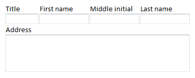
You can merge cells exactly the way you want using Excel’s own Format Cells command.
- First select all the adjacent cells you want to merge, then right-click somewhere in the area and select Format Cells….
- On the Alignment tab, check the Merge cells option. This will create one big cell from all the cells in your selection.
- Adjust the horizontal and vertical alignment if necessary.
- Verify your cell names. All the names that were used for different cells before you merged them will now apply to the whole merged cell.
- If you’ve merged a cell vertically, i.e. with one or more cells below it, select Wrap text for the text in the merged cell to flow nicely as a multi-line paragraph.
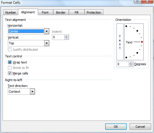
Special considerations for image widget placeholders 
Image widgets like Link Image, Google Map or barcode are represented in Excel using an empty placeholder. The placeholder cannot show the correct image in Excel, but it allows you to position the image correctly within the form and give it the correct size. When you convert the spreadsheet to a web page, the widget replaces the placeholder with the actual image it is supposed to show, e.g. the image, map or barcode.
Before you insert any kind of image widget we always recommend that you merge the cells behind the image placeholder. As you can see in the screenshot below, we merged cells A19:B23 to create a small container for the placeholder. In most cases it works fine anyway but merging the cells makes it much more obvious to both you and SpreadsheetConverter where the image is supposed to go.
To insert an image widget, select the cell where you want the upper left-hand corner of the placeholder to appear. Make the task pane visible. Locate the Widgets tab and click on the appropriate widget icon to insert the placeholder into the selected cell.
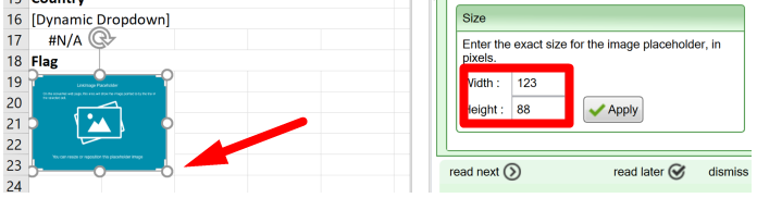
You can drag the placeholder to the best position, and change the size of the widget’s image as it appears on the web page by dragging the placeholder’s handles. In our case, we made the placeholder the same size as the merged cell area behind it. To adjust the width and height to an exact size in pixels, enter your numbers in the corresponding widget settings and click Apply (the widget settings look slightly different for each type of image widget, but you get the picture).
How do I design a spreadsheet to look good as a web page ? 
Read our comprehensive design guide to learn how to design web calculators for a global, mobile audience:
- A large part of your users will be using their phones to use the web page.
- Put the caption on top of each field, not to the left of it.
- Arrange the sections of the calculator or form below each other, or on different tabs.
- For wider examples, you must use responsive design to make the example fit also narrow screens.
- As a desktop user, you may love to analyze data in wide tables with countless columns. This doesn’t work well on phones. You have many options.
- Always test all your calculators with your own phone.
- Assume your calculator or form will be used by an international audience.
- Your calculator may need to handle both metric and US customary units.
- Learn more about the differences in the formatting of date, time and numbers.
- Use only colors that are as far away from each other as possible, using colors that are unambiguous also to colorblind persons.
- Use the table in the design guide.
Optimizing the column width for phone screens 
A column in Excel that has a width of 26 will occupy about half the screen width of most smartphones in portrait mode. As a rule of thumb, you can multiply the width of a column in Excel with 7 to get the resulting column width on the screen, expressed in CSS pixels.
That last part probably didn’t mean anything to you. And yet it’s a very useful thing to know if you wish to design a spreadsheet to exactly match a given screen width without zooming. If you are like most people, you don’t need this exact control of the layout. For you, we have provided an “automatic” option called Fit page to screen width on the Workbook tab. Just tick this checkbox and skip the rest of this section.
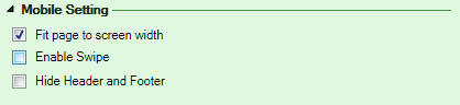
Still curious? Let’s take it from the start.
The screen of a laptop, tablet or phone consists of pixels, the small physical points that together form the raster image on the screen. The density of these pixels directly affects the image resolution – the more pixels per inch, the better the image quality. Changing the physical pixel density usually does not affect the size of the objects on the screen. A phone with twice the pixel density still shows the objects in the same size, otherwise many things on the screen would become too small to see or touch.
This is because web designers can express how big an object is to be on the screen, regardless of the physical pixel density. This is called logical pixels or CSS pixels. As an example, many phones have a CSS pixel width of 360 in portrait mode. This means that an object with a width of 180 CSS pixels would fill half the screen width on all these devices. It would look better on phones with a higher pixel density, but it would be the same size.
In the table at https://www.mydevice.io/#compare-devices you can see the screen width in CSS pixels for many current handheld devices.
And now we’re back at where we started. The width of a column on the web page, in CSS pixels, is approximately 7 times the width of the same column in Excel. So if you want a column to fill half the screen width of a common phone in portrait mode, you should start testing with a column width of 26 in Excel. This is because the width of the phone’s screen probably is around 360 CSS pixels, and half of that is 180, and divided by seven is 26. Or put the other way: a column in Excel that is 26 wide will become approximately 7 * 26 or about 180 CSS pixels wide on the phone’s screen, which is half the width of the most common phone screens in portrait mode.
A word of warning: once you’ve come this far, you’ll probably want to turn on the “auto” setting above anyway, because it also handles device rotation seamlessly. Switch to landscape mode and the contents still fit the now much wider screen. If you don’t enable this setting, your spreadsheet will appear with exactly the same width in landscape mode as in portrait mode, which may leave a lot of unused space to the right.
The browser effect 
When your spreadsheet is converted into web format, you will lose most of the detailed control of the user experience you had when you designed it in Excel. As an example, most web browsers remove spaces as they see fit. If you position text by inserting extra spaces before or after a word, you will find that even though SpreadsheetConverter maintains the extra spaces in the converted web page, the browser simply discards them, which may give a totally different layout to the page.
Once converted into web format, spreadsheets also enter the realm of competing and sometimes incompatible web browsers. No browser is identical to the other, and a web page will inherently appear somewhat different in each browser and device. This is part of the natural behavior of the world-wide web.
When SpreadsheetConverter converts a spreadsheet for the web, it is forced to make certain compromises when it comes to formatting. When compared to the original spreadsheet in Excel, the web page created by SpreadsheetConverter will not be an identical twin regardless of which browser or device you use to view it. In fact, it will look slightly different in every browser, and often different between versions of the same browser. Once again, this is a natural consequence of entering the web environment. In most cases, the result is good enough. Just remember to test your web page in as many browsers and devices as you can.
Learn more 
Some of our tutorials partly focus on web page formatting and layout:
Help: Instant Testing 
Instant Testing lets you quickly test each new version directly after conversion. For mobile devices, just scan the barcode to open the web page.
Instant Testing offers several time-saving services to developers:
- After you convert a form or calculator to a web page, it opens automatically in one or more of your web browsers.
- The converted web page can be directly accessed from other devices on the same network, without uploading it to a web server.
- A link to the just converted web page is provided in the form of a barcode that can be scanned using the camera in a mobile device or laptop to open it.
Introduction 
Automatic preview in your web browser 
Use the Browsers and Conversion Path Option in the Options menu in the Convert section of the ribbon to select what browsers to use for Instant Preview.
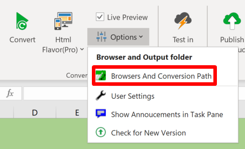
Select one or more web browsers by clicking on their icons – click once to activate a browser, click once again to deactivate. After each conversion, the converted web page will open automatically in all the selected browsers.

The QR code window 
Instant Preview is very useful when you want to test a converted web app in your phone. SpreadsheetConverter automatically generates a barcode, a so-called Quick Response code, that contains a link to the converted web page. Scanning the barcode with a mobile device opens the converted web page in a web browser on a smartphone or tablet. Read more in the QR code tutorial.
To display the QR code for a particular web page in the developer’s environment, just go to the History List and click on the QR icon to open the QR code window.
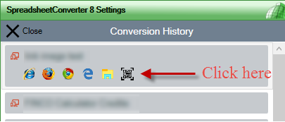
The ThemePreview toolbar also contains a convenient link to obtain the QR code, e.g. if you want to see how different themes change the appearance of a web app in a mobile device.

Remember to use Refresh 
If you are viewing a converted web page from a distance on another device, you only need the address to the Instant Testing device the first time you open the page. If you already have the converted web app open in your web browser, just press the Reload button. It is usually a circular arrow (it looks like a “rotate clockwise” symbol) and it is often located near the website address field.
Ready for production use 
When you have finished testing a spreadsheet, you can of course keep using it from the development environment if all users are on the same network as the developer, and the development system is permanently online.
If you want to make a calculator or web form available outside your own local network, you have to upload the converted web page to a public web server.
Testing in other computers 
The Instant Testing web server in the development workstation attempts to provide the converted web page to any computer or another device on the same network. Copy the link and send it to other devices via e-mail or messaging. You can also take a screenshot of the QR code and forward it to anyone on your local network.
We instruct the firewall to allow access to the Instant Testing server only from Private networks, and we don’t recommend that you open it on Public networks (like at your local coffee shop). If you want to open the firewall to enable Instant Testing also from other secure, in-house networks within your corporate domain, you should open the firewall settings for Inbound connections, and locate the entry for the SpreadsheetConverter Local server. On the Advanced tab, tick the checkbox for Domain, but not for Public.
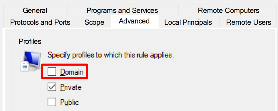
Troubleshooting 
During the installation of SpreadsheetConverter, we install a tiny web server in the development environment that serves the converted web pages to web browsers in the same PC, or to other devices on the same network.
You may be unable to connect to the development environment. In this case, you may get time-out error messages in your web browser saying
- the page can’t be reached or displayed
- the server is taking too long to respond
- the connection has timed out.
You should also check the Messages tab of the task pane for error messages like these from the conversion:
- Local web server error: The server failed to start.
- Localhost Error: the page could not preview from localhost.
All devices must be on the same network 
If you are trying to access the web page in the development workstation from another device, you should double-check that you are indeed connected to the same network as the development workstation. Your device should typically be showing a wifi symbol for the local network – don’t try this with a phone that says it’s connected with 5G, 4G or any other “G” because it probably won’t be able to reach your local devices.
Good:  Bad:
Bad: 
“Localhost” is, well, local 
If the link you have contains the word localhost, it can only be used on the development workstation. To use the link from another computer on the local network, you must replace “localhost” with the local network address to the development workstation. Read more under Determine the local network address below.
Using more than one IP address in the development workstation 
To access the preview web server in the development workstation, other devices need to know its network address. All computers on a network have more than one so-called IP address that can be used to refer to it. Sometimes it’s pretty easy to determine this address, but there are a number of more complex network configurations that we just cannot handle automatically.
- Multiple network adapters: Computer C1 is connected to networks A and B using two network adapters. Computer A1 on network A wants to use Instant Testing on C1, and it needs to use the A interface and address for C1. Computer B1 on network B wants to use Instant Testing on C1, and it needs to use the B interface and address for C1. B1 cannot use the A address since it isn’t even connected to network A and it has no way to communicate with any device on that network. And there have to be two or more QR codes to choose from as well, depending on whether the mobile device is connected to network A or B.
- Active VPN connection: If you are using a Virtual Private Network, it may have established several additional IP addresses for the advanced routing of packages across the VPN connection.
- Internet Connection Sharing: If you are sharing your Internet connection with other users on the same network, there will be special reserved IP addresses for this that cannot be used for Instant Testing or Live Preview.
In cases like these, we must hand the problem over to you, or someone with basic networking skills that can help you determine the correct IP address and firewall settings.
Determine the local network address 
Here are the initial steps to identify the development workstation’s “true” IP address on the local network:
- Open a Command Prompt on the development workstation.
- Type route print.
- The output from route print contains all the different network Interfaces. One of these IP addresses can be used to access your computer from the local network.
- Move to the screen of any computer on the local network from which you want to connect to the development workstation.
- In the link, insert the IP addresses from the Interfaces column above, one by one, until you find one that works from that particular device.
Hint: the link should eventually look something like this:
During a Live Preview session:
http://192.168.59.2:8888/livepreview/weekly-time-card/weekly-time-card.htm
For Instant Testing:
http://192.168.59.2:8888/l/weekly-time-card/weekly-time-card.htm
Antivirus issues 
Some overly anxious antivirus and Internet security programs may incorrectly identify portions of our product as malware. We frequently see false alarms related to the node-ssc.exe or node.exe programs, in particular from Bitdefender. If you get such messages, you may have to whitelist the program or disable the antivirus program completely while using SpreadsheetConverter.
Read more on the help page for Internet security software.
Firewall issues 
The only traffic going into your network should be things that you or someone else asked for, like web pages, downloaded files or e-mail. Your network has one or more “firewalls” that prevent unauthorized network connections to your devices. If someone on the outside attempts to connect to a suspicious program in your laptop, it’s probably a bad thing. One of the firewalls should detect and prevent this intrusion.
Most networks have a primary firewall in or near the network’s outermost router or gateway, the one that connects your network to the public Internet. Many network devices like computers and smartphones also have their own firewalls. The firewalls monitor the applications to see what network ports they open, and allow data to flow through authorized connections. Unauthorized connections are terminated.
When we install our small web server in the development workstation, we do attempt to register it properly in the Windows Firewall. In case it doesn’t work as expected, you must adjust the firewall to enable access to the built-in web server, or our preview functionality will be unavailable. Please follow the instructions below.
The built-in server automatically finds a free incoming port, so the port number may change. You must ensure that the firewall is open for all ports that are opened by node-ssc.exe, not only the port number it is currently using.
The instruction on how to change these settings in the Windows Firewall are below. Please follow the instructions relevant to the version of Windows that is used in the development environment. If you use a third-party firewall, please follow the corresponding instructions in the applicable documentation.
Windows 8 and Windows 10 
These instructions apply to the development workstation, e.g. the PC where you have installed SpreadsheetConverter, if it’s running Windows 8 or Windows 10.
- Open the Windows Firewall control panel.
- In the left pane, click Allow an app or feature through Windows Firewall.
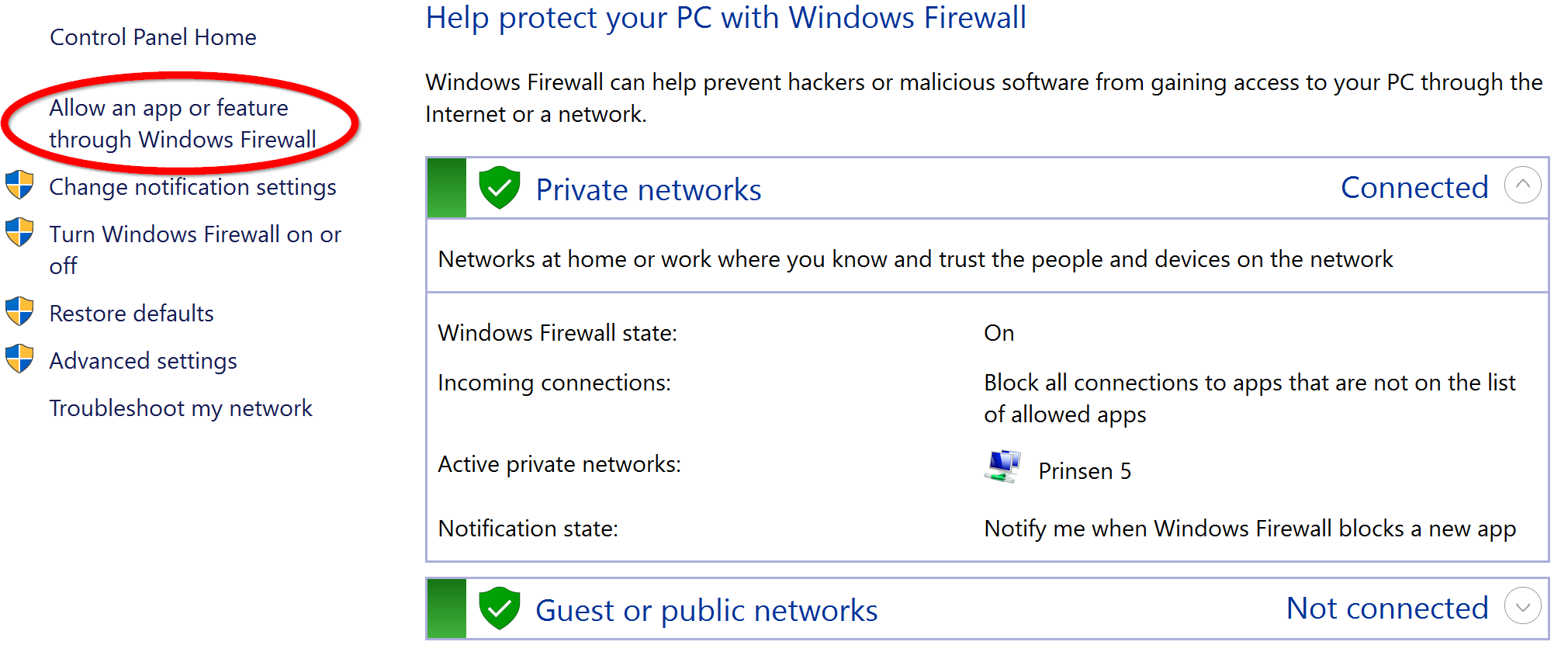
- Click Change settings at #1 on the screenshot below. If you’re prompted for an administrator password or confirmation, type the password or provide confirmation.
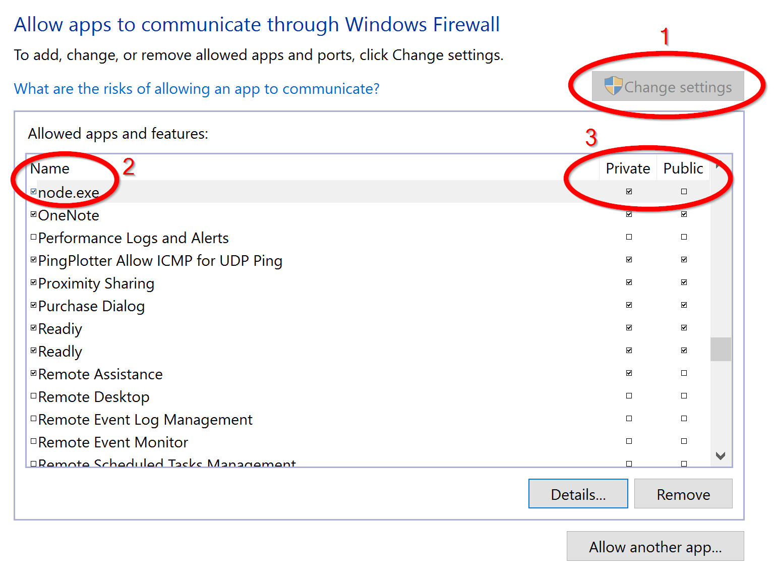
- Select the check box next to the node-ssc.exe or node.exe program at #2 on the screenshot above.
- Select the check box for Private at #3 on the screenshot below. Deselect the check box for Public so that the web server is not accessible for users of insecure public networks.
- Click OK.
- Close the Windows Firewall control panel.
- Move to the cell phone, tablet or laptop that you were using to test the online calculator. Refresh the calculator web page in the web browser – the page that got the time-out error message – and it will probably load correctly now. If it doesn’t, don’t hesitate to contact our Help Desk.
Windows 7 
These instructions apply to the development workstation, e.g. the PC where you have installed SpreadsheetConverter, if it’s running Windows 7.
- Open the Windows Firewall control panel.
- In the left pane, click Allow a program or feature through Windows Firewall.
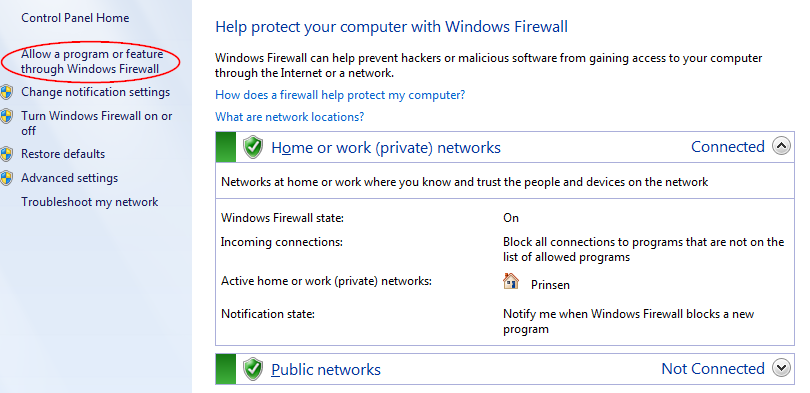
- Click Change settings at #1 on the screenshot below. If you’re prompted for an administrator password or confirmation, type the password or provide confirmation.
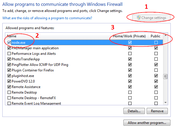
- Select the check box next to the node-ssc.exe or node.exe program at #2 on the screenshot above.
- Select the check box for Home/Work (Private) at #3 on the screenshot below. Deselect the check box for Public so that the web server is not accessible for users of insecure public networks.
- Click OK.
- Close the Windows Firewall control panel.
- Move to the cell phone, tablet or laptop that you were using to test the online calculator. Refresh the calculator web page in the web browser – the page that got the time-out error message – and it will probably load correctly now. If it doesn’t, don’t hesitate to contact our Help Desk.
Interactive charts 
Interactive charts 
Follow these instructions to enable and create interactive charts in Excel spreadsheets converted to web format with SpreadsheetConverter.
If you have a chart in your spreadsheet, SpreadsheetConverter will automatically try to create a similar chart in the converted web page. We support all the major chart types and features.
Supported chart types 
Note that some chart types are available only in the Professional edition.
Professional edition 
- Bar and Stacked Bar charts
- Column and Stacked Column charts
- Line and Stacked Line charts
- Area and Stacked Area charts
- Radar charts
- Pie charts
- Doughnut charts
- Scatter charts
Standard edition 
- Bar charts
- Column charts
- Pie charts
Supported chart features 
- Chart Title
- Legend
- Axis Title
- Secondary Axis
- Grid Lines
- Line Color
- Line Style
- Data labels
- Font Formatting
- Logarithmic series
Enabling interactive charts 
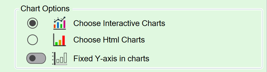
The Chart options are located on the Workbook tab of the task pane.
The Choose HTML Charts option may remain in effect for spreadsheets most recently converted with older versions of SpreadsheetConverter. To switch to interactive charts, just select Choose Interactive Charts.
To see the effect of changing these settings, convert the spreadsheet again.
How to interact with the charts 
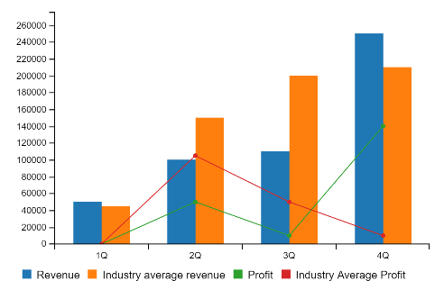
The interactive charts allow you to highlight one of the series just by hovering your mouse above its label.
In the screenshot below, we just held the mouse pointer above the Revenue series’ label. As you can see, the other three series faded out to let you focus on the highlighted series.
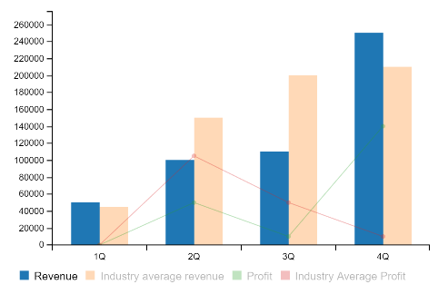
If you find some of the series distracting, just click once on the series labels and the series will be hidden. In the chart below, we simply clicked on the Industry average revenue and Industry Average Profit labels to hide them. Click on each label again to make the series visible.
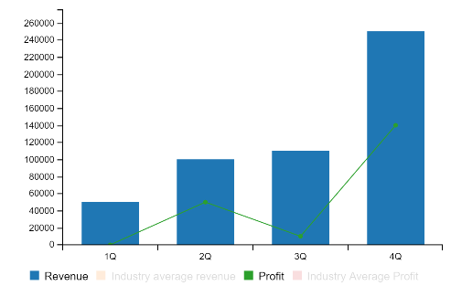
If you want to try this for yourself, create a Combo chart in Excel. In Excel 2016, it is at the bottom of the All charts tab.
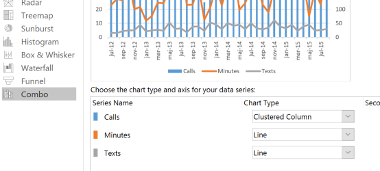
You can also download our example spreadsheet just to see how charts can look in converted web pages.
Test an example of interactive charts
Download the example spreadsheet
Downloading a chart in image format 
Interactive charts contain a convenient download link that allows you to save the chart as an image file.
Learn more 
Some of our tutorials partly focus on interactive charts:
Introduction to using widgets 
Introduction to using widgets 
Use widgets in your spreadsheet to improve the functionality and appearance of the converted web page. This help page introduces you to widgets and their common features.
SpreadsheetConverter provides an extensive selection of graphical widgets that makes your web page more appealing and easier to use. Use pre-formatted text fields, dropdown lists and calendars to improve the quality of the input data. Use Google maps and dynamically selected images to show your website visitors where you are, and what it looks like.
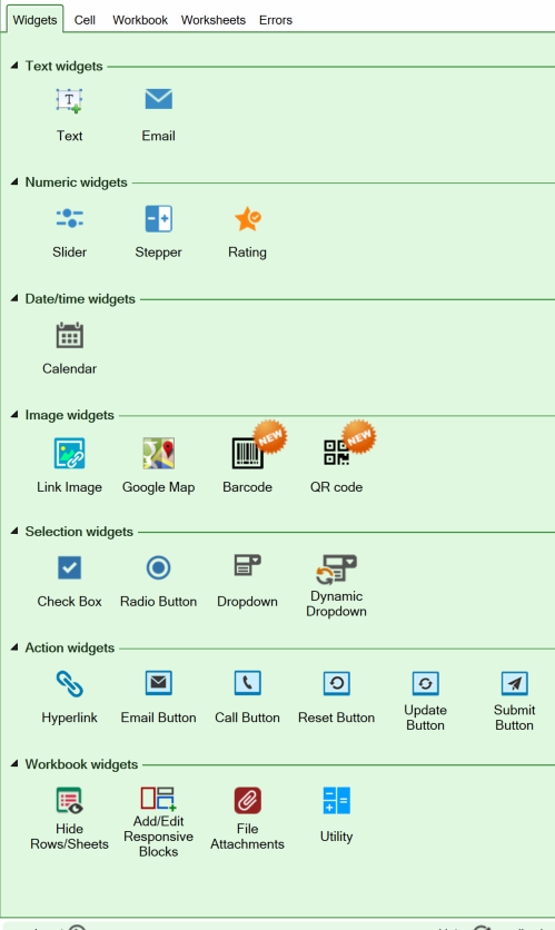
Widgets are inserted in the spreadsheet from the Widgets tab of the SpreadsheetConverter task pane in Excel. Select the cell where you want to insert the widget; then select the type of widget from the task pane. An options dialog appears, in which you can specify the detailed settings for the widget.
Most widgets are fully visible only in the web environment, even though you manage them in an Excel spreadsheet. To review the visual appearance of a web page containing widgets, you must convert your spreadsheet for the web and verify the result in a web browser.
Widgets make the converted web page look better 
In general, spreadsheets have a strict user interface. Often, it’s just letters and numbers arranged in rows and columns. When spreadsheets like these are converted to web pages, they look dreadful (we really should call them dreadsheets).
SpreadsheetConverter re-uses any existing graphical elements already present in your spreadsheets. An input field containing true/false values automatically becomes a checkbox, and a dropdown list created with Data > Validation > List becomes a dropdown list also in the converted web page.
To help you create a more appealing user interface, we took a step further and created a toolbox of user interface widgets that makes it much easier to use your calculator or web form:
- Don’t write a date – pick one from a calendar.
- Don’t list the things you need, tick the checkboxes next to the items you want.
- Show an image of the wallpaper the customer is considering, in the selected color.
- Use single- or multichoice menus for selection.
- Use steppers or sliders to change a numeric value in real-time.
- Use the Ratings widget to make it easy for your visitors to rate products or services.
- Create an unlimited number of text fields in any size or shape you like.
- Add a Google map to help people find your store.
- Insert an e-mail button for those you want to contact you.
Special widgets for small touchscreens 
When using a mobile device, it can sometimes be difficult to enter data with proper formatting. Many mobile devices offer optimized keyboards for special data types, e.g. a numeric keypad. Some browsers offer data entry templates like date pickers, and even provide syntax validation.
The Text widget can request that the user’s web browser provides additional assistance when entering certain types of input. Your mobile users will be grateful for this help.
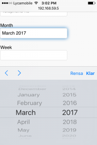
The browser provides the user assistance 
A word of caution, though: Although we can request this assistance from the browser, we cannot guarantee that the browser properly supports all input types, or that your users appreciate the help the browser is trying to provide. As an example, the full syntax for an e-mail address is very complicated and you can expect poorly coded web browsers to reject unusual but formally correct e-mail addresses such as john.smith(comment)@example.com or john.smith@[IPv6:2001:db8::1] while cheerfully approving obviously incorrect e-mail addresses such as john.smith.@example.com.
Users don’t like having correct input data flagged as incorrect by poorly tested web browsers. If possible, please test the advanced input types carefully before you implement them.
Examples of touchscreen widgets 
- E-mail address – “.com” and other top-level domains may be added to the keyboard by the browser, and the e-mail address may be validated for proper syntax.
- Telephone number – a special telephone keyboard may be provided by the browser, and the field contents may be validated.
- Month – a date picker for year and month may be provided by the browser in the default language and regional format set for the device.
- Week – a date picker for year and week may be provided by the browser in the regional format set for the device.
- Number – a numeric keypad may be provided by the browser, and non-numeric content in the field may be flagged.
- Date – a date picker may be provided by the browser in the default language and regional format set for the device.
- Time – a time picker may be provided by the browser in the regional format set for the device.
Insert widgets 
The Widgets tab of the task pane contains all the widgets available in your flavor of SpreadsheetConverter. If you have a license for more than one flavor, always remember to select the flavor you will convert with before you start adding or editing widgets. That way you get the widgets and settings that are appropriate for the flavor you will be using when you convert the spreadsheet to a web page.
You can open the Widgets tab using the Insert Widget shortcut in the ribbon.
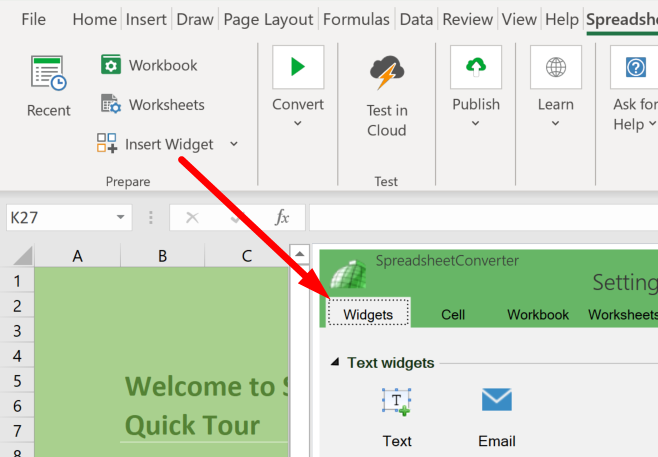
To insert a widget in a cell. select the cell where you want the widget to appear, then click on the widget’s icon on the Widgets tab in the task pane. A settings window appears to let you set the options for the widget you have selected, e.g.:
- For dropdown lists, listboxes and radio buttons you enter the various different choices that the user can choose from.
- For sliders and star ratings, you set the range of values, e.g. 0-100 for a slider or 1-5 stars for a rating.
If you later need to modify these settings, just select the cell again and the settings page for the cell’s widget will appear in the task pane.
In version 10 or later, you can select multiple cells and insert the same type of widget in all selected cells with a single click. Regardless of how you insert widgets, you must still select them one by one to edit their properties.
Widget defaults 
Many of the widgets have an initial value by default. You can usually override the default initial value by inserting a value in the cell of the spreadsheet in which you placed the widget, so if you type Hello into a cell that contains a Text widget, the widget will initially have that value, too.
When the form is converted to a web page and opened in a web browser, most widgets are open for user input. The person that is using the form can override the initial values by changing the value of each widget.
We have tried to document the default value for every widget in their respective help pages. Here is a summary:
- Text: empty, override by typing a value into the spreadsheet cell.
- Slider: the minimum value for the slider, override by typing a value into the spreadsheet cell.
- Stepper: the minimum value for the stepper, override by typing a value into the spreadsheet cell.
- Rating: 0, override by typing a value into the spreadsheet cell.
- Calendar: the current date, override by typing a date into the spreadsheet cell, or removing the default altogether.
- Check box: FALSE (unticked), override by typing TRUE into the spreadsheet cell.
- Radio buttons: the first choice in the list, override by moving one of the other choices to the top of the list.
- Dropdown: the first choice in the list, override by moving one of the other choices to the top of the list.
- Utility: the value returned by the formula in the cell.
Pre-fill form fields from the link 
You can pre-fill many form fields from the link to the form. As an example, if the link to the form contains a language code (/form.htm?lang=sv), it will be preserved by the form if your form has a text field named lang, and it will be forwarded with the form when the form is submitted for processing.
Read more about filling form fields from the link.
Common settings 
Required 
Some widgets can be set as Required, meaning that the user of a web form must do something with the widget before the form can be submitted. Here are some of the actions required by the user for the most common widgets, when they are set as Required:
- Text: must enter text.
- Radio buttons: must “press” one of the buttons.
- Dropdown: must move the menu away from the option that is selected by default.
Hidden 
Developers use Hidden fields when they want a cell to be visible in the spreadsheet, but not in the converted web page. This allows them to provide information in the form without showing it in the form. As an example, if you use a cell to keep track of how long it took a user to fill in a form, you may want to hide this calculation. Even though a field is hidden, it’s contents are forwarded with the form when the form is submitted for processing. It is also common that developers use hidden form fields when pre-filling content from the link (see above),
Cell name 
For electronic forms, it is much easier to process the form if all input fields have names. You can name your cells in the widgets or give them cell names in Excel.
Widget names can start with numbers or an underscore, which is required when integrating with products like Salesforce.
You must assign a name to a cell if you want to pass data into it from the link to the form (see above).
Make widgets look good 
Merge adjacent cells 
Widgets use the same row/column layout as the rest of the spreadsheet. Many of the widgets may require more space than the default row height and column width in Excel.
As an example, if you use a dropdown list, a listbox or radio buttons to select a city or state name from a list, you probably want the widget to be wide enough for the longest name in the list. If you don’t, your flavor of SpreadsheetConverter must either wrap the longer names over more than one line (e.g. for radio buttons), or truncate the names after the allotted width (e.g. for dropdown lists).
If a widget is too big to fit within its cell’s height and width, the corresponding row and/or column may be widened automatically, depending on the web browser. This will probably harm the layout of your spreadsheet in an unpredictable way.
To make room for a large widget you can use Excel’s own Format Cells command to merge the cells in a cell area into one. First select all the adjacent cells you want to merge, then right-click somewhere in the area and select Format Cells…. On the Alignment tab, check the Merge cells option. This will create one big cell from all the cells you selected. Adjust the horizontal and vertical alignment if necessary.
In the example below, four columns and three rows, in total twelve cells, were merged for the Address multi-line text widget.
Move or copy a widget 
Cell widgets can be moved using Ctrl+X and then pasted into one or more other cells with Ctrl+V. You can also drag the cell and drop it in its new location.
Starting with version 10, cell so that any received data is easier to decode. When you cut-and-paste a widget into a single cell you just move it to a different location under the same name, but a copied widget always needs its own unique name, and whenever you paste a widget into more than one cell you should go through them and give them their own names.
Regardless of how you insert widgets, you must still select them one by one to edit their properties. Copying widgets by selecting a cell and pressing Enter or using AutoFill (Fill Down/Fill Right) is not supported. In version 9 and older, copying a cell in which a widget resides will only copy the cell’s contents, not the widget or its settings.
Remove a widget 
Most widgets have a Remove button. To remove a widget, select its cell and click Remove on the widget’s settings page.
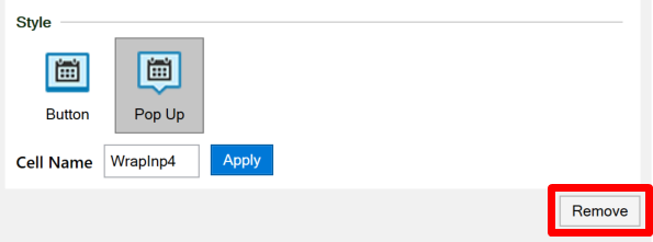
If the task pane doesn’t open automatically, click on the Edit widget button in the SpreadsheetConverter ribbon.
If the cell still isn’t empty, it may contain a default value or a comment. Right-click on the cell and select Clear Contents from the menu to clear the cell.
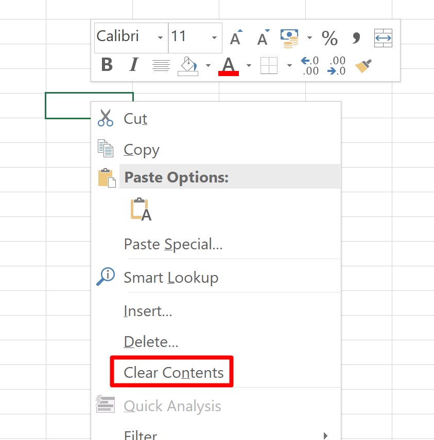
Finally, since we use Data Validation for some widgets, you may also have to go to Excel’s Data tab, locate the Data Validation settings and click Clear All and then click OK.
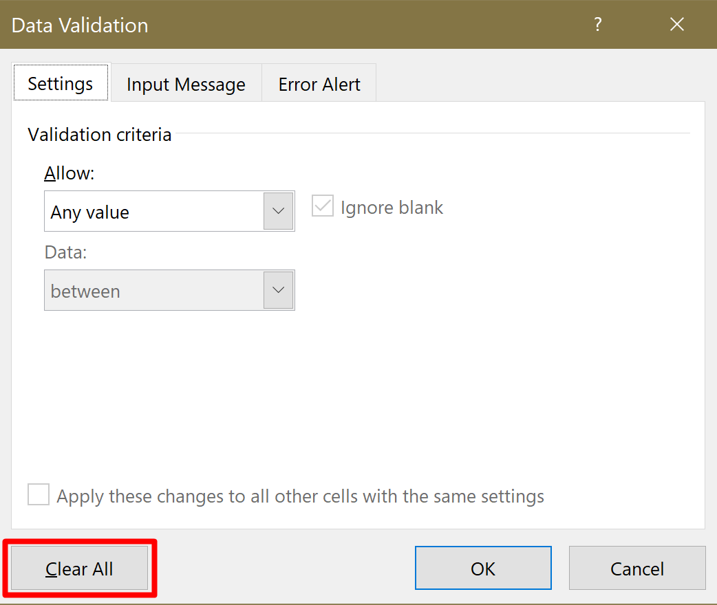
Known issues 
Some widgets must be inserted one by one 
From version 10, most cell widgets can be inserted into two or more cells with the same operation. The Dropdown, Dynamic Dropdown and Radio widgets still need to be inserted one by one.
Image widgets cannot be copied 
Widgets that use image placeholders like Link Image and Google Map may appear to support copying, but you are not copying the actual widget, only making a twin of its image placeholder. All these twin placeholders will always show identical content, since they are controlled by the same widget definition.
Learn more 
Detailed descriptions of each widget in the desktop flavors
Detailed descriptions of the widgets in the iPhone/Android flavor
The Link Image widget 
The Link Image widget 
The Link Image widget allows you to show different images on the web page depending on cell values or formulas. Now you can build advanced imaging applications where an image on the screen changes with the values in a web form or calculator.
When you paste static images into the cells of an Excel spreadsheet, the same image is always shown, regardless of what’s going on in the spreadsheet.
With the Link Image widget, you can freely switch between multiple images. Just provide a link to the right image in a cell in your spreadsheet. The image link can be picked from a list or dynamically created by cell values and formulas in the spreadsheet. When the link changes, the Link Image widget automatically shows the right image.
This is useful in many situations:
- Show an electrical plug in the right format for a particular region.
- Provide the right map to a visitor depending on the visitor’s choice of transportation.
- Show the right image of a new sofa after the user has selected the right fabric, colors and all the other options for it.
- Allow the user to switch between overview and detail photos of a circuit board that is being configured in the spreadsheet.
Widgets like Link Image provide web-related features that are not available in plain Excel. If this is the first time you use widgets, you should first read the introduction to using widgets. Most important is that widgets are fully visible only in the web environment. You don’t see much of them until you convert the spreadsheet to a web page.
Example: see the flag for any country 
The below example comes from the membership application tutorial, where the Link Image widget plays an important role.
In this membership application form, the new member selects a home country using a Dynamic Dropdown widget. A link to the new member’s country flag is saved with the form. Thanks to the Link Image widget, the right flag is also shown at the bottom of the form.
Try it for yourself! Select your home country in the form and watch the flag change.
If you enter all the required data in the form, you can press the Submit button and see what a form like this looks like when someone submits it to you.
Disclaimer: Working with country data is complicated. Some countries may be more disputed than others. Some countries may have a different official name than you think. Our source for country codes and official country names in English is Wikipedia. Our source for country flags is Flagpedia. For countries without a flag in Flagpedia, we show the flag for the United Nations. Over time, the source may divert from the copy used here. We regret if any part of this tutorial offends you, including the list of countries and their flags.
Make an inventory of the image links 
Upload all the images 
Any images you wish to use with the Link Image widget must be published on the web before you can use them in the widget. The widget does not store the images it is showing; all images are fetched live from the web.
All your web users must have access to all the images. If one or more images are protected by a login, you should put the form behind the same login so that all the users can view the images you link to. If your image is reserved for particular “friends” or “members”, you must ensure that all your users indeed belong to this category – otherwise, they won’t be eligible to view the images.
We recommend that you store the images in such a way that you can use secure links (beginning with https) to the images. If you use an electronic form with our Advanced Submit Service, any secure images will be included in the PDF file for each submitted form.
Create a hidden worksheet 
Many widgets require background data that you don’t want to make visible on the web page. In most situations, it is very convenient to have one or more background data sheets to keep this data in. Using the Worksheets tab of the task pane, we can easily mark this worksheet as hidden in the converted web page.
Create the image links 
If you have a list of static image links, you can just paste these into the hidden worksheet.
You can also construct dynamic image links any way you like, using any available cell values and formulas:
="https://example.com/products/" & prod_num & "/images/" & image_num & ".png"
Working with themes and design 
The electronic forms that you create with SpreadsheetConverter don’t have to be plain. You can use all the formatting options in Excel like column width, background color and character size. Excel doesn’t know much about web page design, so we added a simple Theme Designer to give you full control over the formatting of the web page.
Below is a further developed version of the same membership application form. We just changed the background color to brown, and the foreground color to white.
Design the form 
Obtain the image link 
The spreadsheet must contain a full inventory of the links you will be using with the Link Image widget. Usually, you will save the image links in a hidden background worksheet.
Here is an example of background worksheet with a list of countries, and a link to the flag for each country.

In the example above, the image links are in column F. The index to the table is the two- or three-character ISO code in column A and B, respectively. You can also use a numeric code in column C or the country name in column D.
To find the right image link, and provide it to the Link Image widget, it is common to use the VLOOKUP function in Excel:
=VLOOKUP(A16;Countries!$D$1:$F$251;3;FALSE)
What the formula does:
- It defines a temporary cell range, D1:F251 in the Countries background worksheet.
- It takes the country name, set by a dropdown in cell A16, and looks it up in the leftmost column of the cell range to find the right row.
- From this row, it returns the value of column 3 in the cell range (column D counts as 1, E as 2 and F as 3). So, the formula returns the image link in column F for the right country name in column D.
Insert the Link Image widget 
Image widgets like Link Image, Google Map or barcode are represented in Excel using an empty placeholder. The placeholder cannot show the correct image in Excel, but it allows you to position the image correctly within the form and give it the correct size. When you convert the spreadsheet to a web page, the widget replaces the placeholder with the actual image it is supposed to show, e.g. the map or barcode.
Before you insert any kind of image widget we always recommend that you merge the cells behind the image placeholder. In most cases it works fine anyway but merging the cells makes it much more obvious to both you and SpreadsheetConverter where the image is supposed to go.
To insert a Link Image widget, select the cell where you want the upper left-hand corner of the placeholder to appear. Make the task pane visible. Locate the Widgets tab and click on the Link Image widget icon to insert the placeholder into the selected cell.
Select the cell that will contain the image link 
When you insert the Link Image widget into a cell, you also need to tell it in what cell it can find a link to the image it is expected to show. Set the Image Reference to the cell that contains this link. In this example, the link is returned by a VLOOKUP formula in cell A17.
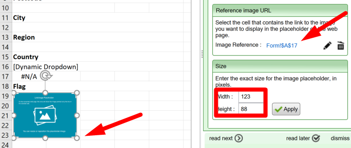
Adjust the size of the placeholder 
You can drag the placeholder to the best position, and change the size of the image as it appears in the web page by dragging the placeholder’s handles. In our case, we made the placeholder the same size as the merged cell area behind it. To adjust the width and height to an exact size in pixels, enter your numbers in the corresponding widget settings and click Apply.
Note: the Link Image widget never distorts the images. If you have a lot of images in various sizes, you can still specify a maximum width and height here. Each image will be resized proportionally to fit entirely within the placeholder.
Conclusion 
The Link Image widget provides a convenient way to display an image on the web inside a placeholder on the web page. The source is a table of image links, usually stored on a hidden worksheet. You can use any static or calculated value in the form or calculator to look up the right image in real-time as the user works with the web page.
Learn more 
Some of our tutorials partly focus on the Link Image widget:
Help: Live Preview 
Technology supporting the creative process 
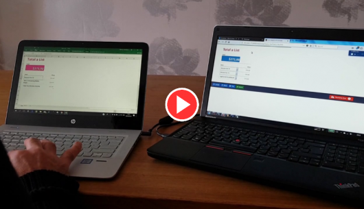

While you edit a spreadsheet in Excel, your changes appear also in a live web page in a separate web browser window. This rapid preview of the converted web page speeds up development and enhances the creative process.
With SpreadsheetConverter, you always see what the converted web page looks like. The preview windows are kept in constant sync with your Excel session and automatically updated every time you save your work in Excel.
As you move back and forth between editing – checking – editing – checking, the only thing holding you back will be the speed of thought. The constantly live preview makes you inclined to test different ideas and to move forward using trial and error. Since any change in Excel automatically appears on the web page, you can gradually refine your design while having the full attention of a tool that is really supporting you in this creative process.
Unlimited previews, unlimited devices 
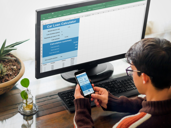

There is some delay due to the complexity of transforming your layout and formulas from Excel to web format, but the automatically updated web page preview still saves a lot of time since you continue to develop the spreadsheet, uninterrupted by the process of converting it for the web.
If your workplace has more than one screen, it’s usually most convenient to use Excel on one screen and show the live preview on another. If your development environment doesn’t have multiple screens, you can use any old laptop or tablet to show the live preview and just put it next to your primary screen.
You can open as many preview windows as you like; both in the development environment, in other computers on the network, and in iPhone and Android mobile devices. Yes, you can preview the office and mobile versions of the web page at the same time, including the effects of our innovative responsive design.
Using Live Preview 
Verify that Instant Testing works 
Before you enable Live Preview, you may want to run a normal conversion and verify that the converted web page opens in one or more of your web browsers. You should also scan the QR code to verify that the development environment is accessible also from other devices on the network. We have assembled some troubleshooting advice on the help page for Instant Testing.
Activate the preview windows 
To enable Live Preview for a spreadsheet, tick the checkbox and press Convert.
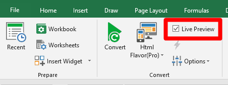
When you activate Live Preview, the spreadsheet is automatically converted to web format and opened in all the web browsers designated for Instant Testing. All preview windows are live and update themselves automatically every time new changes are saved in Excel.
The preview process is managed by a small web server inside the development workstation – the same web server that we use for Instant Testing, and you can connect to it from any device on the local network. The live preview requires very little in terms of computing resources.
If your workplace has more than one screen, it’s usually most convenient to use Excel on one screen and show the live preview on another so that you can just glance at the preview to see the progress you are making.
If you accidentally close or can’t find one of these predefined preview windows in the development workstation, go to the Options menu in the ribbon and click Reopen Live Preview Windows to have them all opened again.
The Live Preview toolbar 
During Live Preview, a progress indicator appears in the title bar of the preview tab in the web browser. The Live Preview toolbar appears in the top right-hand corner of the browser. You can cancel the conversion from the toolbar, or copy the link or QR code to the preview.
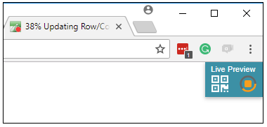
Sending the preview link to someone else 
To see how the web page currently looks also in other desktop or laptop computers, just copy the link from the Live Preview toolbar on the development workstation and forward it to any other user on the same local network. It’s a one-time job, since all previews immediately become live, updating themselves along with the spreadsheet.

You can open an unlimited number of Live Preview windows, both in the development workstation and in an unlimited number of other devices, simply by re-using the preview link or QR code. These preview windows work just like the predefined ones but are unknown to Live Preview. Selecting Reopen Live Preview Windows in the Options menu of the ribbon will only reopen preview windows in the development workstation, and only in the web browsers selected for Instant Testing. To reopen a preview window in another browser or device, re-use the preview link or QR code.
Use the QR code on mobile devices 
If you want to see a live preview on a mobile device you can also click on the QR code symbol in the Live Preview toolbar. This will display a QR code that you can scan with the camera of your mobile device to open a preview window. You can also take a screenshot of the QR code and send it to someone else.
The mobile device must be on the same local network as the development workstation. Turn off the automatic lock or sleep timer on the phone or tablet if you want the display to stay lit until the device is disconnected from the live preview of the editing session. There is a help page about scanning QR codes.
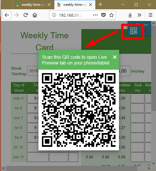
Always end with Save and Convert 
Live Preview does not replace the Convert button. At the end of each editing session:
- Press the Pause button in the SpreadsheetConverter ribbon to inactivate Live Preview.
- Uncheck the Live Preview checkbox.
- Save your spreadsheet in Excel.
- Press Convert on the SpreadsheetConverter menu to create a final, stable version of the web page.
- If the web page is ready for publishing, upload it to the web.
Troubleshooting 
If you run into problems with firewalls or antivirus programs, please follow the instructions on the help page for Instant Testing.
Known issues 
- Live Preview requires the Professional edition of Windows.
- You can only use Live Preview for spreadsheet files in your local file system, not online files that you edit via OneDrive links etc.
- Please turn off Autosave in Excel before you activate Live Preview. Live Preview does not support Autosave.
- The source spreadsheet for Live Preview must be in the xlsx file format. The legacy xls format is not supported.
- You can use Live Preview for only one spreadsheet at a time. Before you enable Live Preview for a spreadsheet, turn it off for all other spreadsheets.
- Turning off Live Preview does not close the browser windows it has been using.
The Print sheet 
The Print sheet 
If your users need to print some of the information in a form or calculator, you may provide a specially formatted print sheet that looks better on paper than just a plain print or screenshot of the web page.
SpreadsheetConverter allows you to create a separate layout just for printing. Typically, such a print sheet just copies information from other cells in the web form, using a more printer-friendly layout.
You designate the print sheet on the Worksheets tab of the task pane. If you have created it specifically for printing, you may also want to hide the print sheet.
The need for a separate print sheet 
Let’s face it – spreadsheets were never easy to print. Excel invites you to design in a landscape format that often becomes too wide for most printers.
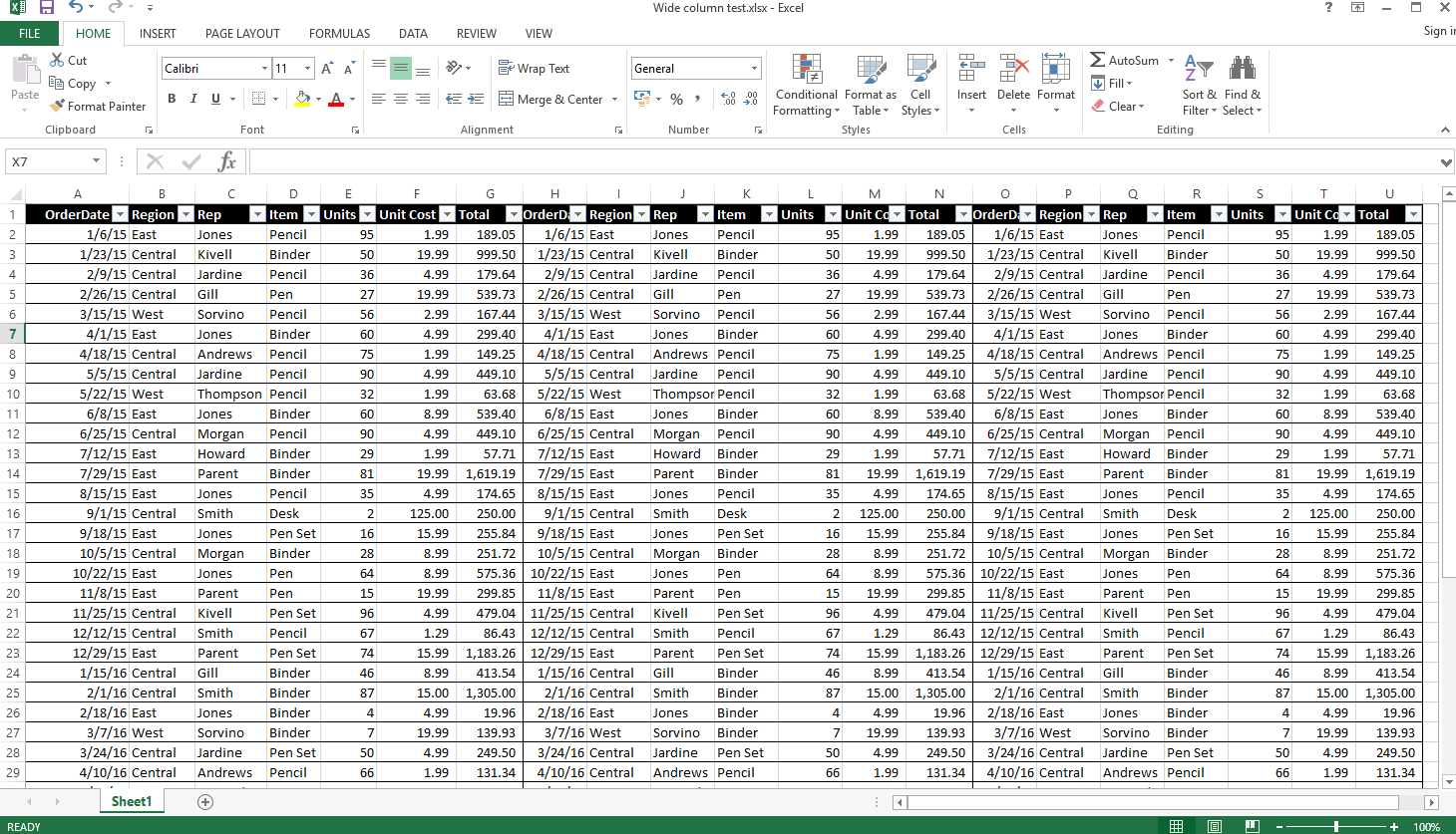
Web pages can be tricky to print, too. They can be designed for legibility, which means there is a lot of guidance and helpful information. There can be excessive use of color and graphical symbols that isn’t optimized for printing.
If you are viewing a web page that uses responsive design for easier viewing on a narrow screen, printing it may create less than optimal results where only the left-most portion of each page is used.
To help you overcome issues like this, we designed the Print Sheet option. A print sheet is just like any other worksheet – you add text and formulas to it so that it contains the information you want to print. You can format the print sheet so that it fits the kind of printers you intend to use it with.
Using a print sheet 
Let’s assume you have a little “wizard” as we call them, a web form consisting of multiple steps.
The first step asks for some information, after which the user presses Next.
The second step asks for some other information, then Next.
There is also a third step in the wizard.
Printing this form would require three printed pages, with very little information on each page.
But when we press Print, the printed output actually looks like this:
This is because the form has a print sheet designated for it on the Worksheets tab. The print sheet is not visible on the web page but automatically used when printing.
The layout of the print sheet is simple, it just aggregates the contents of the three wizard steps into one page.
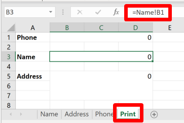
The Print sheet does not have to be special in any way, it can be just any tab in the browser that is the only part of the page you ever want to print.
Details 
Printing operations 
SpreadsheetConverter supports three printing operations:
- Print All – prints all worksheets separately, without using the print sheet.
- Print This – prints the current worksheet, without using the print sheet.
- Print – prints the print sheet. If a print sheet hasn’t been selected, it prints the current worksheet.
If you initiate the print operation from the web browser with the Print menu option or the Ctrl-P keyboard shortcut, it corresponds to the Print operation in the list above.
Create the print sheet 
In Excel, you create a print sheet just like any other worksheet. Just click on the small plus sign to the right of the rightmost worksheet tab.
Name the print sheet 
You can give a print sheet any name you like, as long as it follows our general guidelines. Double-click on the tab name to change it. To reorder the tabs, just drag them to the positions you want.
Select the print sheet 
You select the print sheet by clicking on the corresponding printer symbol on the Worksheets tab. Only one worksheet can be selected as the print sheet. To unselect a currently selected print sheet, click on the printer symbol again.
A print sheet is not hidden by default, but if you have created it specifically for printing it’s unlikely that you want the print sheet to be visible in the web page. You can hide it using the left-hand column, like in the example above. During the development of the print sheet, we recommend that you leave it visible so that the formatted result is visible in the Live Preview.
Fill the print sheet with content 
The print sheet can be any sheet in the workbook. To create a separate print sheet just for printing, you can copy content from the visible, web-formatted worksheets to the hidden print worksheet. Just enter an equal sign in the field, switch to the other worksheet and click in the cell you want to copy.
In the example below
- we selected cell B3 in the Print sheet
- clicked on the Name tab
- selected cell B1
- pressed Enter.
Use Wrap Text for multiline text fields 
To print a multiline text field properly in a merged cell, ensure that you have enabled the Wrap text setting for the merged cell.
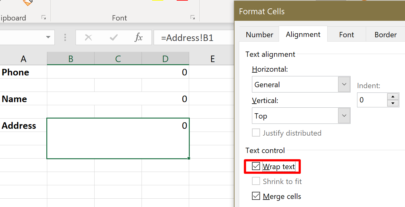
Format a print sheet 
To format the page, you just use the ordinary Excel formatting options and use Live Preview to verify the result on the screen.
For last-minute adjustment of the page width and height, we recommend that you use the print preview option in your web browser to see the page when it has been formatted for printing.
When you have done most of the design work, you may want to hide the print sheet using the settings on the Worksheets tab.
The QR code widget 
Help: QR code widget 
Users can scan QR codes on your web page to follow links, make calls or send e-mails
The QR code widget 
QR Codes make it easy to store a lot of information in a small space. The code can be scanned to identify a person, a location or an object. QR codes are often used on smartphone screens.
Now you can encode any data in your spreadsheet in the form of a QR code. The QR code widget allows you to scan large amounts of information directly off a phone’s screen, from a laptop or in printed form.

QR codes are images with a two-dimensional matrix that is often scanned by or displayed in smartphones. If users see a QR code during a self-guided tour, they can scan it with their phone’s camera to get more information about a significant object, either by listening to a voice recording or by reading a web page.
Since QR codes are square, they fit the phone’s screen well both in portrait and landscape mode, which have made them popular as linking tools, like the link to one of our example calculators above (scan it with your phone now!). QR codes can also be used for marketing purposes and in discount coupons.
Of course, QR codes can be also used for identification purposes like any standard barcode, and were actually initially developed to track parts in vehicle manufacturing.
For QR codes, we initally support the following code formats:
- Text – the encoded text will be input into the active input field.
- URL – the encoded link will open in the default web browser.
- Call – the encoded phone number will be dialed automatically by the phone.
- E-mail – the encoded e-mail address will be used as the recipient of a new e-mail inside the default e-mail client.
Adding a QR code to your web page 
The QR code widget uses two cells in the spreadsheet, one for the source data and one for the generated QR code. To create the widget, select the cell where you want the upper left-hand corner of the QR code. Open the task pane and select the Widgets tab. Scroll down to the QR code widget. Click on the icon to insert the widget into the selected cell.
The QR code format 
The widget can generate the QR code in different formats. Select the format you want in the Format section of the widget properties.
The source data cell 
The content of the QR code will be taken from one of the cells in the spreadsheet. The source data cell can contain a static value or calculate the QR code contents with a formula. Static and calculated values can be concatenated.
To select the source data cell, click on the Select a cell button, click on the source data cell and then click OK. You can also type a cell reference into the text box and press OK.

The QR code size setting 
A QR code is always square. The size of the QR code on the page is defined by the Size setting. The QR code in the screenshot would be generated as a 150 by 150 pixel matrix.
The QR code placeholder 
When you insert a QR code widget in a cell, a placeholder appears. Each actual QR code is generated starting from the upper left-hand corner of the placeholder.
When you edit the spreadsheet in Excel, the placeholder will not reflect the current value of the source cell. In the example below, the source data is in A1, but if you scan the code below you will find that a QR code placeholder in Excel always points to our website www.spreadsheetconverter.com. In the converted web page, the QR code always correctly shows the current value of the data source.
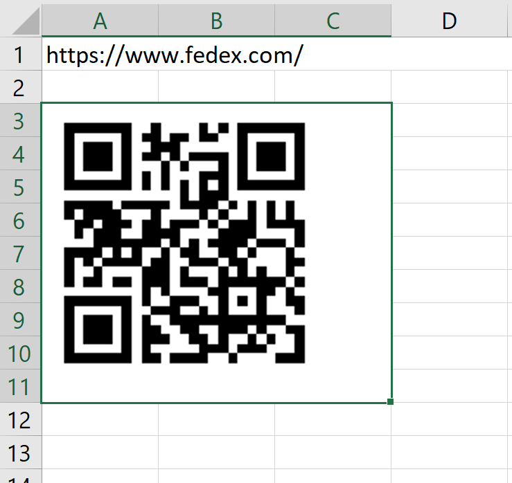
When you work with widgets that use placeholders, you will often get a better result if you merge all the cells behind the placeholder. This enables the converter to better determine the size of the widget as it will appear on the web page. In the example above, we have merged cells A3:C11 to make it easy to align other objects on the page with the image generated by the widget.
The size of the placeholder in Excel is based on your settings for the QR code widget. The best way to change the size of the placeholder is to edit the settings. You can also drag the handles of the placeholder to adjust it. The resulting width of the placeholder will be used for both the height and width of the square QR code.
Data validation 
You need to validate the data used with a QR code 
The QR code widget does not validate any part of the code you provide. If the source data for a QR code is typed manually into a form, you must validate it before you use it to generate a QR code.
- Text QR codes have a maximum length of 2,331 characters, according to the specification (version 40 Binary data with correction level M). You must ensure that the source data isn’t too long, either by testing the length of it using =LEN(qrcode) or by truncating it with =LEFT(qrcode, 2331).
- URL QR codes contain links, usually to web pages. You must verify that the link is a valid URL.
- Call QR codes contain a tel: link as described in https://www.ietf.org/rfc/rfc3966.txt. When dialing with digits, it is always a good habit to ensure that the source data contains the country code, or add one by default. Note that some countries allow Phonewords, i.e. letters in phone numbers; with the alphabet mapped to different digits. In the USA, dialing 1-800-FLOWERS is the same as dialing 1-800-3569377. A QR code can also be used for making Voice Over IP calls where the subscriber is identified by a character string.
- E-mail QR codes must contain a valid e-mail address. The easiest way to ensure this is to use the special E-mail widget in the cell where the e-mail address is typed.
Apple Wallet 

The Apple Wallet offers a convenient way to store and use tickets, membership cards, discount coupons etc in iPhones and Android devices. Many of these passes use QR codes to identify the holder. You can generate your own Apple Wallet passes in-house, or you can use an external API provider.
Getting started 
Getting started 
This is the quick start guide for SpreadsheetConverter. We hope it will get you started converting Excel spreadsheets to live, calculating web pages.
Welcome to the SpreadsheetConverter Quick start guide. It contains the most basic things you need to know to get started with the program.
What do I need to use SpreadsheetConverter? 
- You need a blog or web site where you can upload and publish the web pages you have created with SpreadsheetConverter, so that people can view them in their web browsers.
- You need a Windows PC with Microsoft Excel to create the spreadsheets that SpreadsheetConverter converts to web pages. For more information on technical requirements, visit the flavor comparison page.
- You need to download and install the SpreadsheetConverter add-on for Microsoft Excel according to the instructions below. You may test the program for free for 30 days. If you want to continue using the program or if you want to publish a converted web page, you must buy a license.
If you have any problems, continue with the help page for download problems.
How do I install SpreadsheetConverter? 
- Navigate to the download page and download the appropriate version of SpreadsheetConverter.
- Select Open or Run to execute the installation program immediately after download.
- The installation process should start automatically. Otherwise, navigate to the folder containing the downloaded file and double-click on the file name.
- Carefully read through the license agreement displayed on the screen, then indicate that you accept its terms. If you don’t, please terminate the installation.
- The installation program suggests a default location for the program files. In most cases, you should accept the default location. If you are upgrading a previous installation, you must install the new version at the same location as the old version, or uninstall the old version first.
- During installation, the installer will offer to open the firewall for our built-in webserver. You must enable this to use Instant Testing, i.e. to see the result of a conversion directly in your development environment. The web server is also required if you want to use Live Preview to automatically convert the spreadsheet as you save new changes to it.
- When the installation of SpreadsheetConverter is completed, close the installation program.
If you have any problems, continue with the help page for installation problems.
How do I design a spreadsheet to look good as a web page ? 
Read our comprehensive design guide to learn how to design web calculators for a global, mobile audience:
- A large part of your users will be using their phones to use the web page.
- Put the caption on top of each field, not to the left of it.
- Arrange the sections of the calculator or form below each other, or on different tabs.
- For wider examples, you must use responsive design to make the example fit also narrow screens.
- As a desktop user, you may love to analyze data in wide tables with countless columns. This doesn’t work well on phones. You have many options.
- Always test all your calculators with your own phone.
- Assume your calculator or form will be used by an international audience.
- Your calculator may need to handle both metric and US customary units.
- Learn more about the differences in the formatting of date, time and numbers.
- Use only colors that are as far away from each other as possible, using colors that are unambiguous also to colorblind persons.
- Use the table in the design guide.
How do I convert a spreadsheet to a web page? 
- Ensure that Excel is started.
- Open the spreadsheet you want to convert.
- Select the SpreadsheetConverter menu in Excel’s menu bar.
- In the SpreadsheetConverter menu, click Convert.
- After conversion, a Messages tab appears in the task pane. Often, there are only informational messages.
- Normally, the generated web page is automatically opened in your default web browser. You can use the History list to open the converted web page in a web browser or in the Windows Explorer.
- Verify the results of the conversion. If you are unhappy with the results, you should consider modifying the original spreadsheet in Excel before you attempt to modify the converted web page.
For more detailed instructions, read the overview of the conversion process.
If you have any technical problems, continue with the help page for startup problems. Never hesitate to contact our Help Desk.
How do I publish a SpreadsheetConverter web page on the web? 
- Use the Publish to Cloud function to upload the web page. It will give you an iframe that you can paste into the html of any blog or website. If you use the Node.js flavor, you can test the web page by uploading it to QuickNode instead.
- If you want the converted web page physically included in your own web site, transfer it to the same web server as the other web pages in the web site using file transfer, a site management utility or a content management system. This guarantees that the page is physically accessible when requested by one of the users of the web site.
- Link the page to the rest of your site. You will need at least one link to the page so that users can navigate to it.
- We have many useful tutorials about how to integrate a calculating web page with your existing blog or website.
Note: SpreadsheetConverter offers a free trial period. Publishing on the web is not included in the free functionality. You must have a paid license for SpreadsheetConverter before you publish converted spreadsheets on the web.
Rules for input files 
Rules for input files 
Your spreadsheet must follow these rules, otherwise we will have problems converting it.
Rules for input files 
For your spreadsheet to convert gracefully into a properly formatted web page, it must follow certain rules that are documented on this help page.
When you create spreadsheets with Excel, there are a lot of rules for what you can put in the file, how big it can be and how you can name it. When we later convert your spreadsheet into a web page, many new rules are inherited from the web environment. We will do our best to warn you about any changes you need to make.
Please contact support if you need help with any of the items below.
File name 
The names of your spreadsheet files cannot contain a Comma. They must start with a letter and cannot end with a space.
There are also a lot of other restricted characters that most people rarely use in file names anyway. If you do, Excel or SpreadsheetConverter will tell you what you need to change.
- Excel does not permit \ / : * ? ” < > | [ ]
- SpreadsheetConverter does not permit ‘ , ! @ ^ + { } $ # %
- The WordPress plugin only permits A-Z a-z 0-9 – _
- If you want to publish your calculator using Publish to Cloud which uses external cloud storage suppliers, other naming restrictions may apply.
There is a maximum length for your spreadsheet’s file name but it changes with the circumstances so we’ll just tell you if your file’s name is too long.
Wordsheet name 
Worksheet names must start with a letter.
The name of a worksheet cannot end with a space or contain certain other restricted characters.
You cannot use a worksheet name that starts with a cell reference in the R1C1 notation. Example: “C5_Overhaul” is an invalid worksheet name.
Excel allows you to use 31 characters in a worksheet name, and so do we.
Cell name 
Excel cell names can contain letters, numbers, periods, and underscores, and the first character can also be a backslash. Excel does not allow spaces in cell names.
A cell may only have one name. If named cells are merged, the merged cell has more than one cell name, which is not allowed. Cells with more than one name will be flagged and the conversion terminated.
Many strings cannot be used as cell names because they already are standard cell references. Perhaps you never thought of naming a cell “B2” but it won’t work if you try. “R2C2” is another way of referring to the same cell and cannot be used as a cell name either.
Less obvious are probably “Bad1”, “Sec60” or “Qty1000”, which all are valid cell references. The maximum limit for the number of columns in a spreadsheet is increased now and then in new versions in Excel, and a combination that is valid today may become invalid in two years’ time in a future Excel version. In short: avoid cell names that only consist of letters followed by a positive integer – always put an underscore in-between, as in “Qty_1000”.
The converter reserves some cell names for its own internal use. You cannot use any of these names in your spreadsheet. If you do, we will let you know.
Worksheet size 
Max 1,000 rows 
We will only convert the first 1,000 rows of your spreadsheet. If you are in a free trial period, there will be additional restrictions.
Worksheet content 
There are a few things that we cannot convert for you.
Unsupported functions 
There is a list of the Excel functions that we support, The Professional edition supports more functions than the Standard edition.
Chart sheets 
We cannot convert a worksheet that only contains a chart.
The task pane 
The task pane 
The task pane is where you do much of your work with SpreadsheetConverter. It lets you add graphical widgets and set options for the converted web page.
Showing the task pane 
To show/hide the task pane, click on the dotted symbol on the vertical separator.

Shortcuts in the ribbon 
The task pane uses tabs for its different sections. You can go directly to one of these tabs using the shortcuts in the SpreadsheetConverter ribbon in Excel.
The Workbook shortcut opens the Workbook tab.
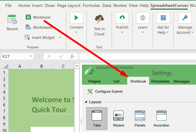
The Worksheets shortcut opens the Worksheets tab.
The Insert widget shortcut opens the Widgets tab.
If there is a widget in the current cell, the Edit widget shortcut opens the Cell tab with the settings for the widget in the cell.
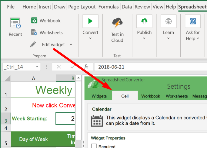
The Messages shortcut opens the Messages tab.
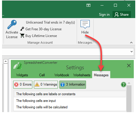
The task pane is pretty wide and can occupy a significant portion of the screen in Excel. When you don’t need it, you can close it by clicking on the X in its upper right-hand corner.
Show/hide task pane in version 9 and older 
In older versions, the Task Pane section of the SpreadsheetConverter menu allows you to Show the task pane when you need it and Hide it when it’s no longer needed.
The Worksheets tab 
On the Worksheets tab, you select the worksheets that will be visible as tabs in the converted web page. You can hide worksheets that only contain long tables of internal lookup data. Using a special Print Sheet, you can optimize the layout of the web page for printing.
The Widgets tab 
If you click on the Widgets tab you get a list of the various graphical widgets you can insert into the spreadsheet.
The Cell tab 
Click on the Cell tab to adjust the settings for the widget in the currently selected cell.
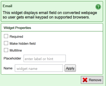
The Messages tab 
After each conversion, any error messages are available on the Messages tab of the task pane. Shorter messages in the upper section link to more detail below.
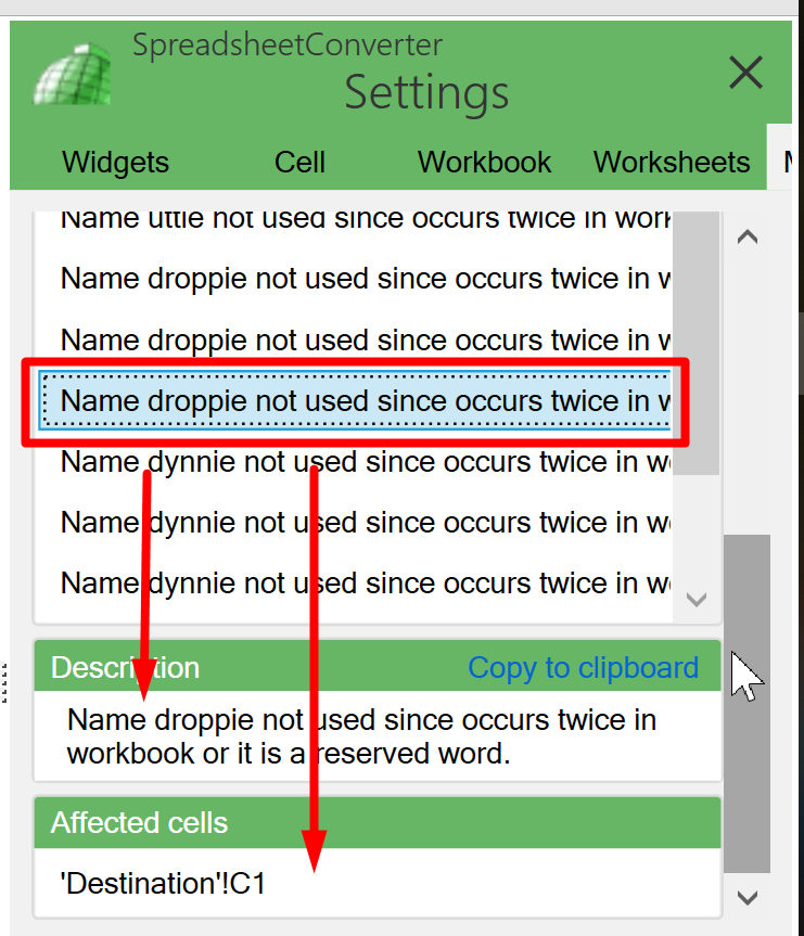
This tab was called Errors in version 9 and older.
Adjusting the task pane 
To change the width of the task pane, hold the mouse over the vertical separator but below the five dots until it turns into a double arrow, then click and drag the vertical separator left/right to match your requirements.
Testing in Excel 
Testing in Excel 
When you’ve created a new calculating web page in Excel, you may want to test it already in Excel before you convert and publish it on a server. Here are a few useful tips.
Excel offers a few simple tools to enhance the value of spreadsheets. The Scenario Manager can test the calculator with a number of predefined values. With Goal Seek, you can decide the result you want and have Excel use trial-and-error looking for the perfect input data.
Scenario Manager 
One of the most powerful uses for the Scenario Manager is regression testing, i.e. to ensure that you don’t introduce errors in existing functionality as you develop a complicated calculator. If the output of your formulas is essentially linear, you can probably just throw in a few values and see that the result matches your expectations, but what if the formulas have thresholds that fundamentally change the behavior of the calculator for certain value ranges? As an example, a tax calculation can use very different formulas at various levels of income. In such cases, it’s good to prepare a structured set of values to test with and to know the correct result for each value in advance.
In this example, we have a muffins bakery. At the beginning of the day, we can sell blueberry muffins at full price, with a profit of £1.00. As the day goes on, the muffins become less fresh and people start looking for other products. We then reduce the price, which lowers our profit to £0.40 per muffin.
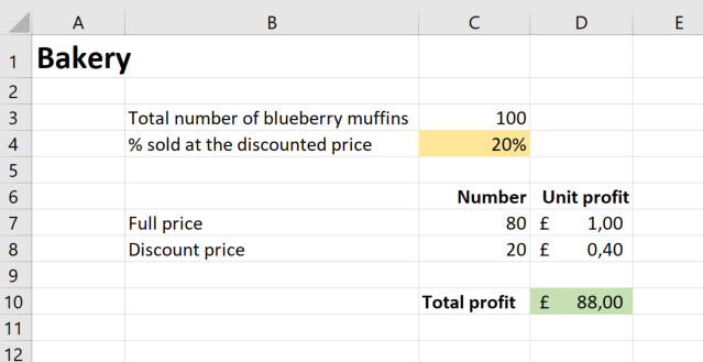
As you can see in the calculation above, if we sell 20% of the muffins at the discount price we have a total profit of £88.00 from blueberry muffins every business day.
Now we want to know how much our total profits from these muffins will decrease if we increase the number that is sold at a discount. To do this what-if analysis, we will use Excel’s Scenario Manager.
The Scenario Manager is started from the Data section of the ribbon, Forecasts group, What-If Analysis menu.
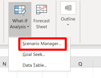
The Scenario Manager window allows you to create the scenarios you want. In our case, we will create five different scenarios with 0%, 5%, 10%, 15%, and 20% of the muffins sold at the discounted price. To add the first of the five scenarios, we click on the Add button in the Scenario Manager window.
We give the scenario a name and select the cell that we want to assign a value to in the scenario.
When you press OK, the Scenario Manager wants to know the value to use for the changing cell C4 in the scenario. For this scenario, the value is 0%.
Now repeat these steps to add the scenarios for 5%, 10%, 15%, and 20%.
To test the calculator with each scenario, select the scenario in the list and press Show. Excel inserts the corresponding value in C4 and calculates the result.
If you want to test all the scenarios simultaneously, click on Summary. Excel asks you which of the cells in the spreadsheet you consider the most important to save for each scenario, the Result cell. In our case, this is the Total profit in D10.
Click OK. Excel inserts the scenario values, one by one into C4, and for each input value, it saves the result value returned in D10. The resulting table is saved as a new worksheet.

You may think that this was much work for something you know several ways to do much quicker. The benefit of using the Scenario Manager is that you can save as many scenarios as you like together with the spreadsheet you want to test. You can perform these tests as often as you like – every time you edit the spreadsheet, if you like – and it takes almost no time. There is hardly any manual work involved even for very extensive testing of the calculator, except during the initial setup.
Goal Seek 
Simply speaking, Excel’s Goal Seek does the opposite of what the Scenario Manager does. Using trial-and-error, Goal Seek goes directly searching for the perfect value that satisfies your request, without showing you all the values that figured in-between. Like with the Scenario Manager, if the output of your formulas is essentially linear, you can probably just improvise a few values and pretty quickly navigate manually to the result that best matches your expectations.
In the complex world of real life, however, there are lots of situations where a result changes direction and suddenly starts to decrease with higher input values. As an example, this behavior is typical of workload calculations, where total productivity first increases with added load, but then starts to decrease when the subsystem is overloaded. Using Goal Seek, you could immediately find the sweet spot for the subsystem, where productivity cannot be increased further.
Using Goal Seek, we will now ask Excel to use the muffins calculator to find out how many of the muffins we can sell at the discounted price and still make 66% of the maximum profit.
The Goal Seek function is started from the Data section of the ribbon, Forecasts group, What-If Analysis menu.
To run Goal Seek, Excel needs to know
- What cell you want to use as the result of the test, in our case the Total result, in D10.
- What value you want the result cell to contain when the goal is reached. In our case, the maximum profit from muffins is £100.00 if they’re all sold at the full price. If we’re willing to sacrifice one-third of that, the goal value is £66.00.
- What value in the spreadsheet you want Excel to vary until it reaches the goal, in this case, the number of muffins sold at a discount, in C4.
Enter these values into the Goal Seek prompt.
Click OK. Excel tries different values in D10 until it reaches the goal value of £66.00 in C4 and then proudly presents the results.
What everybody wants to know now is the input value that gave the goal value as a result. One day, Excel may use the Goal Seek Status window to give us this directly. Until then, we have to look in cell C4 ourselves. We now know that we can sell 57% or more than half of the blueberry muffins at the discounted price, and still make two-thirds of the maximum profit.
The Conversion Process 
Help: The Conversion process 
This is the Online Help page describing the SpreadsheetConverter conversion process.
The Conversion Process 
When you press the Convert button, SpreadsheetConverter creates a new, calculating web page for your blog or website. This Online Help page describes what happens during the conversion process and some of the issues that may arise.
When you convert a spreadsheet to a web page, it is saved in your PC and you can examine the result there using Instant Testing. This Help page describes what’s going on behind the curtains, and points you to other information sources if you want more detail.
To help you publish the web page on the world-wide web, we provide a secure connection to file sharing services where you may share your web page.
Step-by-step 
Setup 
- Start Excel.
- Open the spreadsheet in Excel.
- Navigate to the SpreadsheetConverter ribbon menu.
- Select the flavor or output format.
With Live Preview 
Use Live Preview if you want the spreadsheet converted automatically, every time you save.
- Select Live Preview.
- Click Convert.
- If you are designing a mobile calculator, scan the barcode provided on the Live Preview toolbar.
- Make any last-minute changes to the spreadsheet.
- Save the spreadsheet regularly.
- Check for any messages from the most recent conversion.
- Verify your changes in the updated live preview window(s).
Without Live Preview 
If you feel distracted by Live Preview, or prefer to do all your planned changes before the first conversion:
- Make any last-minute changes to the spreadsheet.
- Save the spreadsheet regularly.
- Unselect Live Preview.
- Click Convert to start the conversion.
- If you are designing a mobile calculator, scan the barcode provided for Instant Testing.
- Check for any messages from the conversion.
- Verify your changes in the Instant Testing window.
For details, please follow the sales tax calculator tutorial.
Upload the converted web page on the web 
After conversion, a web version of your spreadsheet has been stored in the folder designated by your settings. You can publish the calculator online using Publish to Cloud or using our plugin for WordPress.
If you open the History List from the SpreadsheetConverter menu, the converted web page will appear on top. Move your mouse over the file name and select what browser to open the web page in. You can also open the web page folder in the Windows Explorer and see the output file structure.
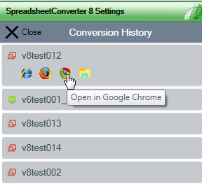
The localhost web server and firewall issues 
When you install SpreadsheetConverter, you also install a miniature web server with the sole mission to host the converted web pages that we store in the folder you have chosen in the Settings. When you convert a form or calculator, or open it from the History list, the web browser will fetch it from this local web server using the reserved address localhost.
If you have any problems viewing converted web pages, it may be that your Windows environment is blocking the access to this local web server. Should this happen, please follow the instructions on how to open ports in the Windows firewall for Instant Testing. You can also contact our Help Desk and they will help you.
Preview the web page 
Using the local web server, you can preview the converted web page and compare it to the Excel spreadsheet you created it from.
If you want to involve other testers, you can do a Test upload to the web using our Publish-to-Cloud service (read more below).
You may want to adjust the formatting or open more fields for input. If you have any problems or questions, please consult the Online Help pages before you contact our Help Desk.
Share the web page 
Publish to Cloud 
SpreadsheetConverter comes with built-in, high-performance web hosting on globally distributed Amazon S3 servers. Use the Test upload location until you like what you see, then begin using it for real from the Production location. Just select Publish to Cloud on the menu to upload a converted web page. With the press of a button, you even get a complete HTML structure to insert the calculator into any blog or website as an iframe.
If you use Node.js, we provide a Test location where you can upload and test a Node.js calculator on our web servers for up to seven days. After that, you must publish the calculator on any public Node.js-enabled web server. For more information, visit the Node.js help page.
Import spreadsheets to WordPress 
If you prefer to host the calculating web page on the same web server as your WordPress site, you should consider using our plugin to import spreadsheets into WordPress.
Any website with FTP 
The Tutorials page contains a tutorial on how to upload a converted calculator or form using the File Transfer Protocol using FileZilla or any other FTP client.
Import an Excel spreadsheet in your blog or website 
Converting spreadsheets to web format makes it very easy to import them into your blog or website. Here are tutorials on how to do this in various popular environments:
- Import Excel spreadsheets and charts in Blogger
- Import Excel spreadsheets and charts in Drupal
- Import Excel spreadsheets and charts in Google Sites
- Import Excel spreadsheets and charts in Joomla
- Import Excel spreadsheets and charts in Squarespace
- Import Excel spreadsheets and charts in Typepad
- Import Excel spreadsheets and charts in Weebly
- Import Excel spreadsheets and charts in Wix
- Import Excel spreadsheets and charts in WordPress with the plugin
- Import Excel spreadsheets and charts in WordPress without the plugin
- Import Excel spreadsheets and charts in any blog or website
Work with more than one flavor 
Most people only work with one format of the web page. If you have a license for more than one flavor of SpreadsheetConverter, be aware that you cannot convert a spreadsheet for more than one flavor at a time. The most recent conversion overwrites the previous also when the flavors are different.
The Excel ribbon menu 
Help: Excel ribbon menu 
This is the Online Help page for the SpreadsheetConverter ribbon menu in Excel
The Excel ribbon menu 
SpreadsheetConverter adds a new ribbon to the Excel menu. This is the online help page for that ribbon menu.
After you have installed SpreadsheetConverter, a new ribbon or menu appears in Excel.
This page describes the new layout of the ribbon menu for SpreadsheetConverter version 10 and later. If you are using an older version, please read the help page for version 9.
If there is no SpreadsheetConverter entry in your Excel menu, please follow these troubleshooting instructions.
When you click on the link, the ribbon shows you many of the controls you need to operate SpreadsheetConverter.
Prepare section 
The Prepare section is where you do most of your work before the conversion.
Recent conversion history 
The Recent file list makes it easy to open or share a recently converted web page. The most recently converted web page is at the top of the list. To the left of the filename is an icon that tells you what flavor was used to create it, i.e. its conversion output format. The timestamp tells you when the file was converted.
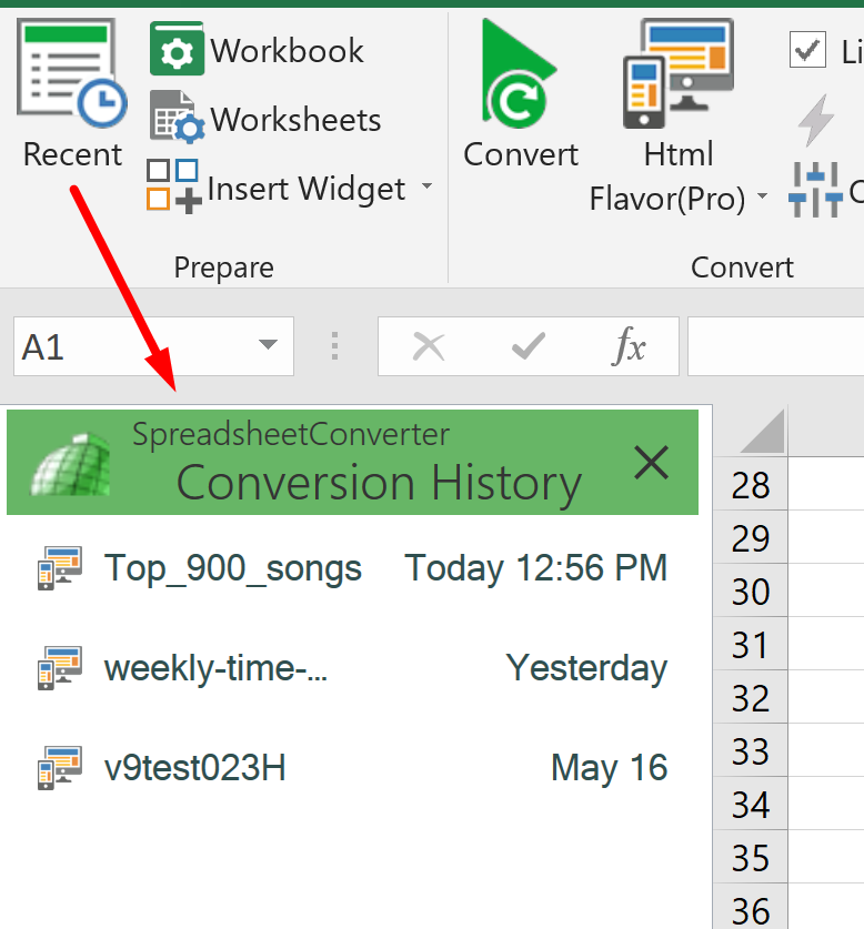
If you hover your mouse pointer over a file in the list, you will see browser icons.
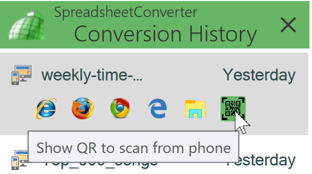
- Click on any browser icon to open the converted web page in the corresponding web browser.
- Click on the Windows Explorer icon to locate the folder that contains the converted web page, e.g. in preparation for uploading it to the web server.
- Click on a QR code icon to generate a QR code for Instant Testing that you can scan with a mobile device to open the corresponding web page with the device’s web browser.
There is a video tutorial for the History List in version 8.
Task pane shortcuts 
Clicking on the shortcuts opens the Workbook or Worksheets tabs of the task pane. If the currently selected cell in Excel does not already contain a widget, you can insert a widget into the current cell.
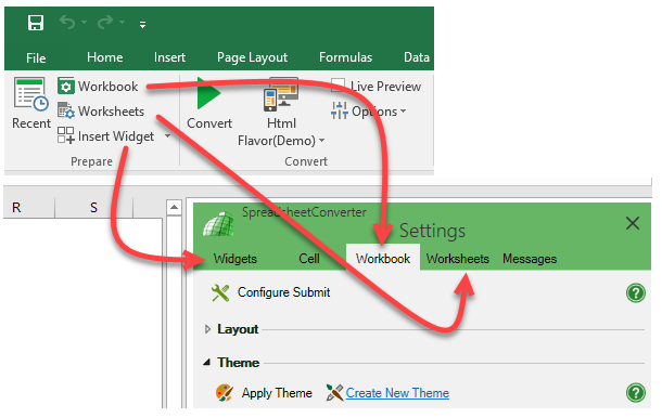
If there is already a widget in the current cell, the Insert Widget button changes into Edit widget to let you access the widget’s settings directly from the ribbon.
The settings for worksheet-level widgets like Hide Rows/Sheets and Responsive Blocks are always accessible directly from the ribbon.
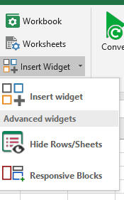
Convert section 
Use the Convert section of the ribbon to select what flavor to use for the conversion, i.e. what format to use for the converted web page. All licenses include the ability to generate standard cross-platform responsive HTML output. You can also buy a license for other flavors.
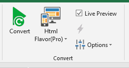
Automatic Live Preview and manual Convert 
Select Live Preview to initiate an automatic conversion of the spreadsheet every time you save it in Excel.
Press Convert to convert the current spreadsheet to a live, calculating web page. There is a tutorial to guide you through your first conversion. If Live Preview is active, a new conversion will automatically be initiated every time you press Save in Excel, updating all preview windows that are connected to the editing session in Excel.
We offer you a free 7-day test of SpreadsheetConverter with access to all flavors in a limited, “demo” mode. You can also request a free 30-day trial license.
After the trial period has ended, unlicensed flavors will no longer appear in the list. If you need a particular flavor, ensure you have a license key for it and that you have activated this license key under Activate License in the Manage Account section of the ribbon. There is an online Help page for license registration.
Note that changing the flavor may affect other settings, e.g. for layout and formatting, and that some widgets may only be relevant in certain flavors.
Options 
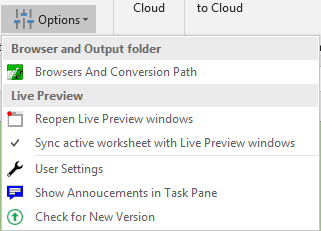
Browsers and Conversion Path Option 
- Click on the button to the right under Choose folder to store webpage and navigate to where you want SpreadsheetConverter to store the web pages it creates. All converted forms and calculators are stored in this folder, even if the source spreadsheets are in different folders. Each converted calculator or form will be enclosed in its own subfolder.
- Your converted web pages automatically open in one or more browsers directly after conversion. Select what browsers you wish to use with this Instant Testing – click once to activate a browser, click once again to deactivate.
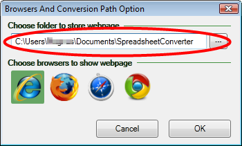
Reopen Live Preview windows 
When you activate Live Preview in the development workstation, it opens a preview window in each browser selected for Instant Testing above. If you accidentally close or can’t find one of these predefined preview windows in the development workstation, click Reopen Live Preview Windows to have them all opened again.

- The new Live Preview windows replace the old ones which now become stale and can be closed. As you can see in the above screenshot of the browser tabs, there is a visual clue on the right-hand active preview window tab that distinguishes it from the left-hand inactive, orphan one. Preview windows without this visual clue will not be updated when the spreadsheet is changed and saved.
- You can open an unlimited number of Live Preview windows, both in the development workstation and in an unlimited number of other devices, simply by re-using the preview link or QR code. These preview windows work just like the predefined ones but are unknown to Live Preview. Selecting Reopen Live Preview Windows will only reopen preview windows in the development workstation, and only in the web browsers selected for Instant Testing. To reopen a preview window in another browser or device, re-use the preview link or QR code.
Show the same tab as in Excel 
Select Sync active worksheet with Live Preview windows to have the preview windows follow the tab you are currently working on Excel. Example: if you select the Shipping tab of the spreadsheet in Excel, this tab will also become visible in all the preview windows.
User settings 
The User Settings are available in version 9 and later. Read more on the help page for the user settings.
Show Announcements in Task Pane 
The announcements in the Notification Center help us communicate new features to you without the use of e-mails, blogs or newsletters. Read more about the Notification Center and how to use it.
Check for New Version 
Before you report any technical problems to us, please ensure that you are using the latest version of the add-in. Otherwise, you may be reporting a problem that has already been fixed. The Check for New Version menu selection will automatically verify the version you have installed, and help you apply any updates.
Test section 
The Test section lets you upload the converted web page to the cloud for testing. You get a fully functional web link that works for 7 days. Send it to anyone in the world to let them test your calculator or web form. If you don’t have a paid license for SpreadsheetConverter, you can only use Test links. There is a Help page for Test and Production upload to cloud.
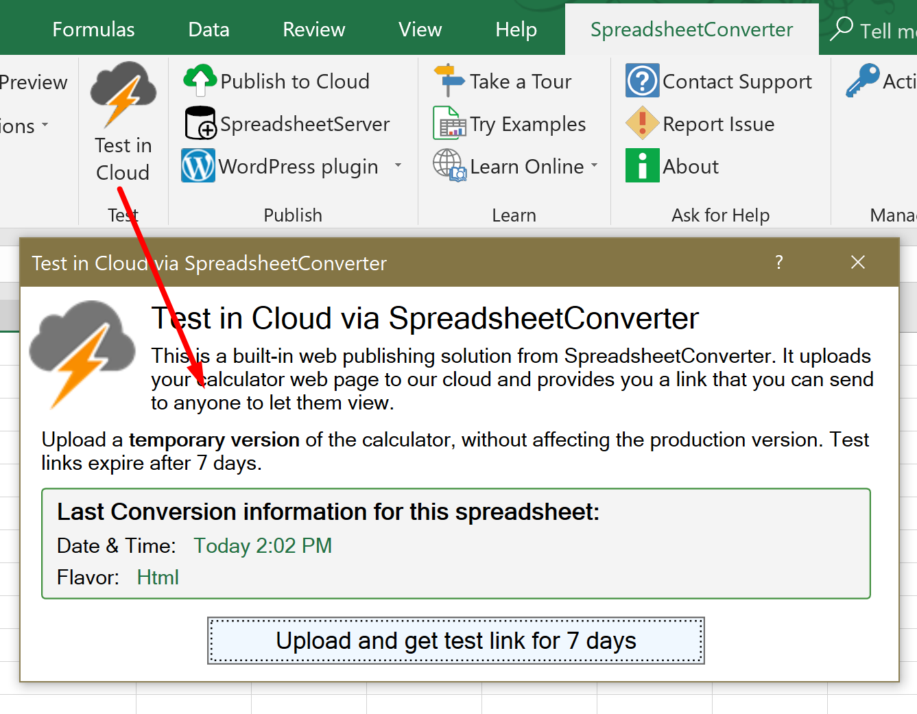
Publish section 
The Publish section of the ribbon helps you publish the converted web page on various external servers. You must convert your spreadsheet before you can share the converted web page.
The choices available depend on what flavor you use, so you may not see all the below in your particular setup.
Publish to Cloud 
When testing is complete and you want to activate the new version of the web page as the live Production version, simply select Publish to Cloud to replace the Production version instead. The basic ability to create production links is included in all paid licenses. Production links are always the same, every time you upload the same spreadsheet, and never expire. There is a Help page for Test and Production upload to cloud.
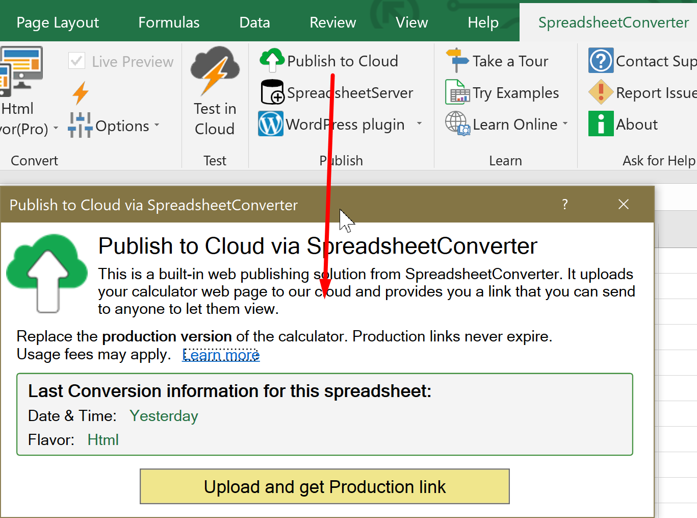
WordPress plugin 
Some flavors include a WordPress plugin which makes it much easier to upload your calculator to WordPress using a plugin.
If you use another content management system, check if there is a shortcut to an integration document for your specific CMS on our website.
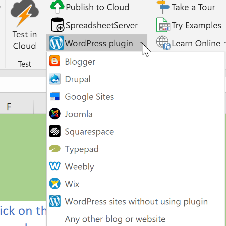
Learn section 
Use the Learn section of the ribbon to gain knowledge and research any problems you might have.
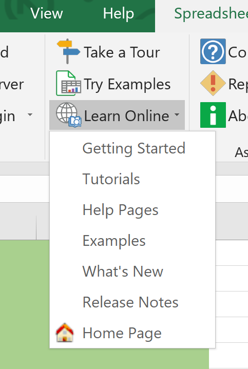
Try some of our examples 
SpreadsheetConverter installs a few examples on your local disk. You can open and test these examples using the Try Examples link in the ribbon.
Press Convert to see what each example looks like as a web page!
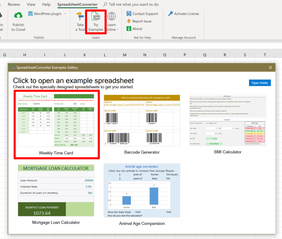
Other learning options 
- Take the Tour, a collection of images and descriptive text that helps you get started.
- There is a direct “getting started” link to the Quick Start Guide.
- You can browse the many Tutorials on the website.
- The “help pages” link takes you directly to the Online Help section of this website.
- Another link opens the directory of online Examples on the web.
- You can visit the News section of the website to see what’s new.
- Every new version has a thick bunch of very interesting Release Notes that you may want to indulge in.
- Follow the “home page” link to visit the start page of our website.
Ask for Help section 
Contact support 
Use Contact Support to open the Contact Support form on the website. This is mainly useful when you want to ask questions.
If you want to report a problem, use Report issue instead.
Report issue 
If you have a problem, use this reporting feature to request help. Adding lots of troubleshooting information is very easy thanks to the convenient checkboxes.
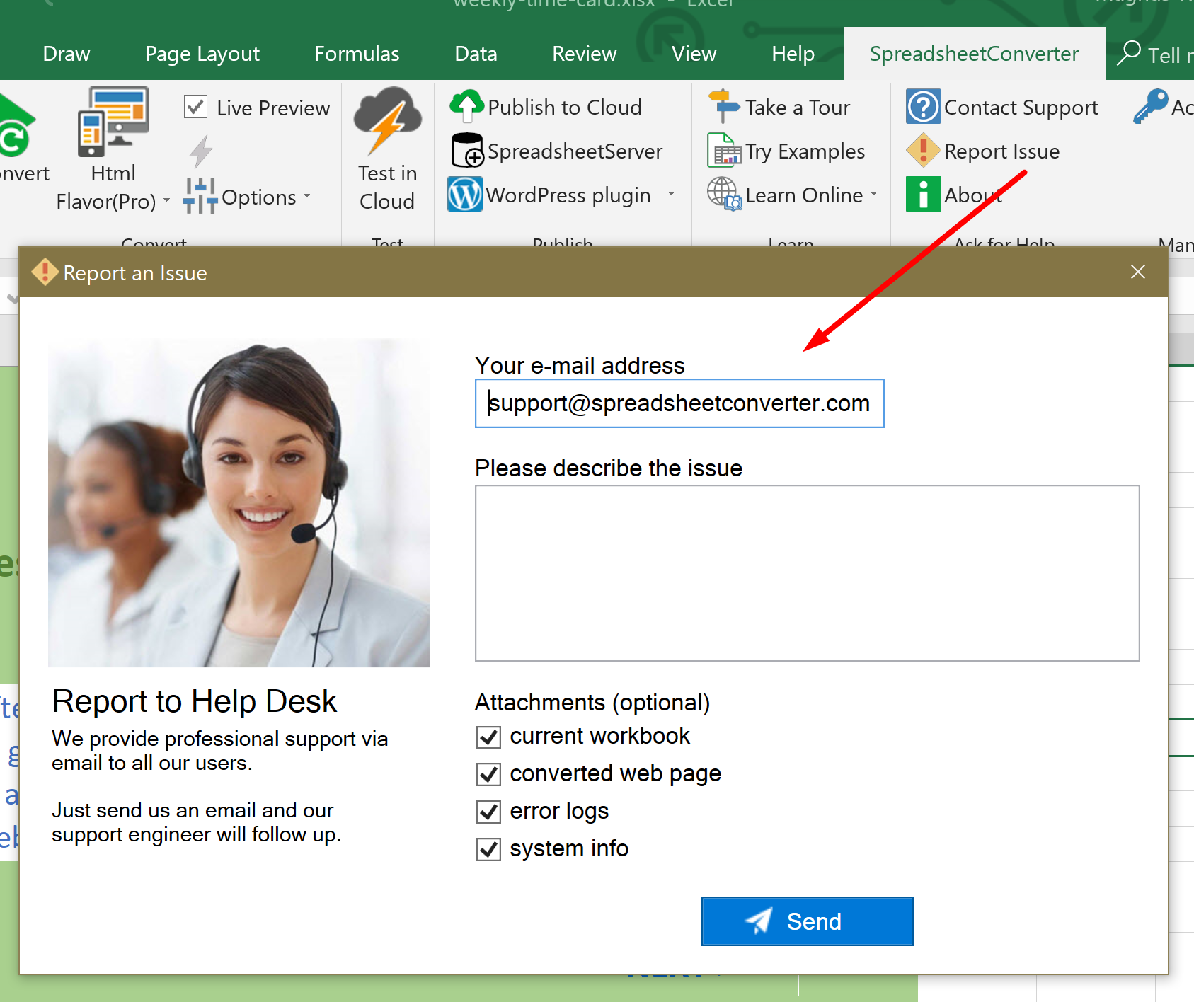
About 
Open the About box to see the currently installed version number. A convenient copy button makes it easy to paste the version number into any question or problem report you send us. The About box also tells you if there is a later version available on the website.
Manage Account section 
Use the Manage account section of the ribbon to register license keys. For upgrades, you may need to register old license keys as well.
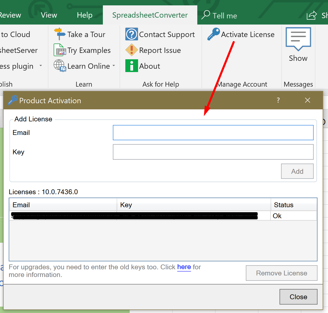
If your flavor is unlicensed, this section instead contains links to get a free 30-day evaluation license or buy a lifetime license for the current version.
Theme Preview 
Theme Preview 
The ThemePreview toolbar allows you to test variations of a theme directly in the web browser.
SpreadsheetConverter uses visual themes to control some of the layout and design aspects of the converted web page. The Theme Preview toolbar lets you tamper with some of these settings directly in the web browser. You can apply different themes, test the Material design, center the page on the screen and change the width of the web page.
The video below shows a few examples of what you can do.
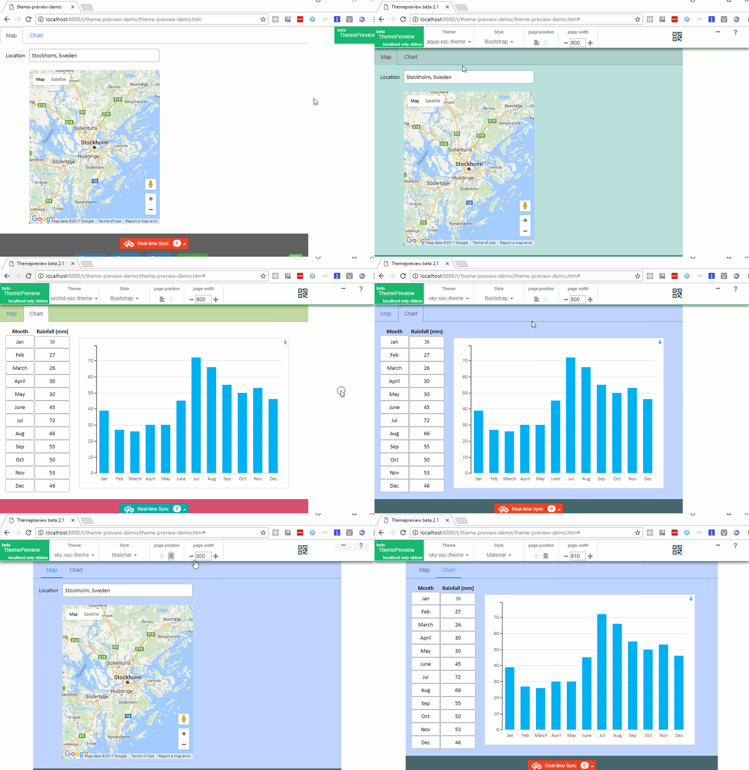
The toolbar is only shown during Instant Testing, i.e. when the address field of the web browser begins with http://localhost. If you publish the page on the web, the toolbar will not be available.
Activating the toolbar 
To activate the Theme Preview toolbar, click on the green box that overlays the upper right of the Instant Preview window.
To reach this help page, click on the question mark in the toolbar.
To close the toolbar, click on the minimize button – it looks like a minus sign.
Compare themes directly 
When you create a theme for SpreadsheetConverter, it is downloaded and saved as a file. You need to install each theme’s file in SpreadsheetConverter to use it with a web page.
With the ThemePreview toolbar, you can switch between the available themes directly in the web browser, which saves a lot of time. Previously, you had to convert the spreadsheet to a web page before you could see a new theme in action.
The themes in the list are the ones that were installed in SpreadsheetConverter before you converted the web page. To compare two or more versions of a design, download and apply them all, one at a time, to the spreadsheet before you convert it. This ensures that all themes become available for testing in the ThemePreview toolbar.
Use the Theme selector to apply a different theme to the web page.
Use the Material design 
There are many ways to design a digital experience. SpreadsheetConverter has for a long time used the popular Bootstrap design. With the ThemePreview toolbar, you can now test what your web page would look like with the Material design from Google.
Use the Style selector to switch between Bootstrap and Material.
Center the page on the screen 
By default, SpreadsheetConverter creates left-aligned web pages. With the ThemePreview toolbar, you can now test what your web page would look like if the contents were instead centered on the screen.
Use the Page position setting to change the horizontal alignment.
Change the body width 
The width of your web page is set by the spreadsheet you are converting. Sometimes you may want the spreadsheet to be more narrow or wide to fit a particular screen width.
Use the Page width setting to experiment with different widths. The width is set in pixels.
Saving the new settings 
Your changes to the settings are saved automatically with the converted web page. If you upload the page to a web server it will use your most recent settings.
If you convert the same spreadsheet again, remember to first apply the theme you decided on. After conversion, you will have to open the Theme Preview again to reapply any other settings.
Preview the web page in iOS or Android 
If you’re happy with a design and want to see what it looks like in a mobile device, click on the QR code symbol in the Theme Preview toolbar.
Point your mobile device’s camera at the barcode to open the web page. There is a tutorial on how to scan QR codes.
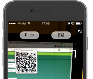
You only have to scan the QR code once to see the changes you’ve made. If the web page is already open in your mobile device, just press the Reload button. It is usually a circular arrow (it looks like a recycle symbol) and it is often located near the website address field.
User settings 
User settings 
The User Settings dialog allows you to use SpreadsheetConverter with other languages than English. It also lets you adjust the advanced conversion settings.
The User settings dialog is opened from the Options menu in the Convert section of the ribbon and contains various options and settings.
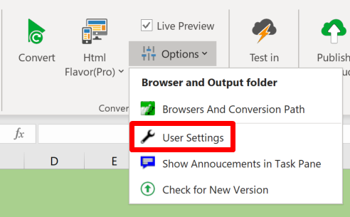
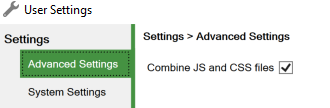
System settings 
- If you’ve changed a lot of things and got lost, and you want to return SpreadsheetConverter to the factory defaults, just press the Reset User Settings button.
- To run a conversion in debug mode (usually requested by our developers), select Enable debug mode conversion. Read more about this setting on the help page for Browser storage.
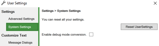
Customize text 
You can translate SpreadsheetConverter to other languages or change the texts it uses with the Customize Texts setting. Select the group in the left-hand pane and edit the texts in the group in the right-hand pane. The new texts will be used for all subsequent conversions, but will not affect already converted web pages.
Read more about translation in the Translation Overview.
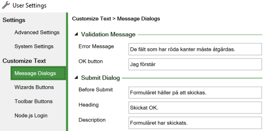
Message dialogs 
You can translate all runtime messages generated by the converter.
Validation Message 
When the user types something into a form field that does not follow the rules for the field, this error message is displayed.
Submit dialog 
These messages are displayed when a form is being submitted.
If you have designated a separate landing page in Configure Submit settings > After successful submit, the After Submit message with its Heading and Description will not appear.
Offline Save 
When forms are being submitted offline, they need to be saved to browser storage. These messages appear when this happens.
Offline Submit 
When the user comes online again, the offline forms can be delivered to the server, with these messages.
Offline Submit Fail 
If the saved forms couldn’t be delivered, these messages may appear.
Wizard Buttons 
If you have a spreadsheet with more than one worksheet and convert it with a Wizard layout, you get buttons to navigate to the Next and Previous step, and a few other buttons. These can be translated here.
Toolbar Buttons 
The buttons in the toolbar can all be translated. The Workbook tab controls which buttons are shown for each calculator or form.
Node.js login 
If you use the Node.js Secure Login feature you can customize the login screen here.
Translation overview 
Translation overview 
Follow these instructions to translate a spreadsheet to another language while you convert it to a web calculator with SpreadsheetConverter.
The SpreadsheetConverter add-in is currently only available in English, but you can use it to convert spreadsheets in any left-to-right language including Greek and Russian.
The converted web pages contain small amounts of standard texts generated by the converter, e.g. warning messages and button labels. You can translate all these using the text customization feature.
Translation of the converted web page 
Considerations when going global 
When you attempt to use a calculator or form in other countries, some things may require particular attention:
- Try to keep the length of the translated text approximately the same as the length of the original text, so that the translation fits the width of the corresponding column or button.
- There are numerous differences in how you format a date, time, number or address. Read more about how you should Design the web page for all your visitors.
Translation checklist 
To create an online spreadsheet that is completely in a non-English language, e.g. Swedish, you need to do the following with the original spreadsheet in Excel, before you convert it:
- Translate the spreadsheet’s file name to Swedish.
- Translate the tab names in the spreadsheet to Swedish.
- Translate the text in all the cells of all the worksheets to Swedish, including any text generated by formulas, functions (like TEXT). Note that Excel generates some localized text strings, most notably the names of weekdays and months in the Long Date format, in the currently selected Windows language. You must change the regional settings in Windows to correct this – read more below.
- Translate the in-cell texts used by SpreadsheetConverter widgets. The Action buttons take their label from the cell they’re in, and the File Attachment widget takes its text prompt from its cell. Note that some texts may have external requirements, e.g. an e-mail message subject, a survey response or a hidden flag that the recipient expects to be in English at all times.
- Translate the text in the SpreadsheetConverter widget settings, e.g. the text for each option in a Dropdown menu.
- Customize the standard texts used by SpreadsheetConverter using the Customize texts settings for the spreadsheet, replacing each English text with its Swedish translation.
- Translate the text generated by other Excel add-ins.
- Translate the Page title in the Workbook settings to Swedish.
- Ensure that all links point to pages in the same language. Example: If the original English calculator has a link to www.example.com/en/calc_help.htm, you need to translate this page as www.example.com/sv/calc_help.htm and change the links in the Swedish calculator to point to this page instead.
- Ensure that any web pages used for the After successful submit, After failed submit and After cancel in the wizard options in the Submit settings are translated into Swedish and properly linked to from any Swedish form or calculator.
- Ensure that forms submitted in Swedish are properly processed after submission, e.g. that they are sent to the an e-mail address where people speak Swedish, or stored properly in a database of responses in Swedish.
- Ensure that the visitor tracking settings are adjusted for the language. You probably want to maintain separate visitor and conversion statistics for each language, and so you should use different settings for your visitor tracking, website statistics, conversion counters, advertising metrics etc.
Regional settings 
Excel and SpreadsheetConverter obey the current regional settings in your Windows environment. Sweden uses ISO-standard yyyy-mm-dd dates, decimal comma and space as the thousands separator. To generate a web page with Swedish date and number formatting and a 24-hour clock, you must change the Windows region setting to Sweden before the conversion.
Help: Use the basic widgets 
SpreadsheetConverter offers you lots of basic graphical widgets that make your web page easier to use and to give it a better appearance. This is the online help page for these widgets.
This is an introduction to the use of widgets in spreadsheets to improve the functionality and appearance of the converted web page. If you haven’t used widgets before, you may want to read the Introduction to using widgets before you continue.
Be aware that most of these widgets have no corresponding representation when used in Excel. Some of them are unfortunately totally invisible in Excel. You have to convert the spreadsheet to web format to see the widget in action.
This page describes the widgets available in the HTML and Node.js flavors. There is a similar page describing the widgets in the iPhone/Android flavor.
Text 
Text fields are mainly used in electronic forms to mark the fields where the user will enter data that is not used in calculations, e.g. a name or an address. You insert a Text field widget by clicking the Text widget in the Widgets tab in the task pane.
You can set different properties for the Text field:
- A Required field requires input from the user. This option is mainly used for electronic forms, where a form must contain a minimum of information to be meaningful. For Text fields, a Required field cannot be empty. If it is, it will not be possible to submit the form.
- Make hidden field is used when you want a cell to be visible in the spreadsheet, but not in the converted web page. This also allows you to provide information to a form processing script without showing it in the form. As an example, if the link to the form contains a language code (/form.htm?lang=sv), it will be preserved by the form if your form has a text field named lang, and it will be forwarded with the form when the form is submitted for processing. Read more about filling form fields from the link.
- Multiline is used to give a text area more than one line and to make it scrollable. Use this option only for text fields that you have made sufficiently large in the spreadsheet, e.g. by merging two or more cells. You can achieve the same result by enabling Wrap Text for the merged cell in Excel.
- Placeholder can contain a text prompt for the field that is visible in the field only when it is empty. As an example, the Placeholder field itself displays the placeholder enter label or hint until you type anything into the field.
- Name your widgets if you want to pass data into them from the link to the form (see above). For electronic forms, it is also much easier to process the form if all input fields have names. You can name your fields in the widgets or give them cell names in Excel. Widget names can start with numbers or an underscore, which is required when integrating with products like Salesforce.
- The default value of a Text field is empty. To provide a different default value, enter text into the spreadsheet cell before conversion.
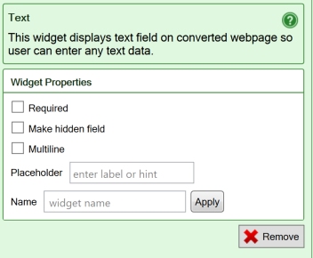
Learn more 
Some of our tutorials partly focus on the Text widget:
Email 
One of the most common and also most complex data validations is to verify that e-mail addresses are correctly written, e.g. that there is only one @ sign, that there is text on both sides of each period etc. The syntax rules for an e-mail address are far too complex to be handled with Excel Data Validation or Excel formulas.
Instead, use the E-mail widget which is a standard text field with built-in validation of e-mail addresses. The field must either be empty or contain a valid e-mail address. If the e-mail address has an incorrect syntax, or if the field is empty but set as Required, the field is considered in error and the form cannot be submitted. This reduces the risk that you receive forms with missing or incorrect e-mail addresses.
The widget only validates the character string in the field; there is no live or online validation that the provided e-mail address actually exists or that someone reads the e-mails sent to it.

The properties for the Email widget are the same as for the Text field:
- A Required field requires input from the user. This option is mainly used for electronic forms, where a form must contain a minimum of information to be meaningful. For Email fields, a Required field cannot be empty. If it is, it will not be possible to submit the form.
- Make hidden field is used when you want a cell to be visible in the spreadsheet, but not in the converted web page. This also allows you to provide information to a form processing script without showing it in the form. As an example, if the link to the form contains a language code (/form.htm?lang=sv), it will be preserved by the form if your form has a text field named lang, and it will be forwarded with the form when the form is submitted for processing. Read more about filling form fields from the link.
- Multiline is used to give a text area more than one line and to make it scrollable. Use this option only for text fields that you have made sufficiently large in the spreadsheet, e.g. by merging two or more cells. You can achieve the same result by enabling Wrap Text for the merged cell in Excel.
- Placeholder can contain a text prompt for the field that is visible in the field only when it is empty. As an example, the Placeholder field itself displays the placeholder enter label or hint until you type anything into the field.
- Name your widgets if you want to pass data into them from the link to the form (see above). For electronic forms, it is also much easier to process the form if all input fields have names. You can name your fields in the widgets or give them cell names in Excel. Widget names can start with numbers or an underscore, which is required when integrating with products like Salesforce.
- The default value of an Email field is empty. To provide a different default value, enter text into the spreadsheet cell before conversion.
Slider 
A Slider allows the user to select a value by moving a handle to a particular position on the widget. Sliders are real-time and cause the entire spreadsheet to be continuously recalculated with each new value of the slider as you move it.
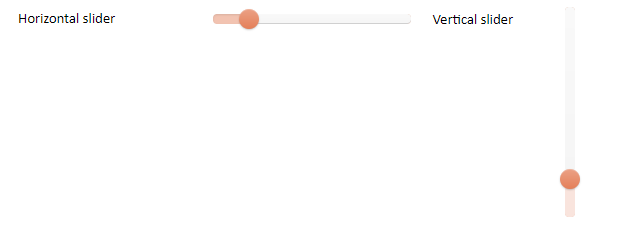
You insert a Slider widget by clicking the Horizontal Slider widget (value increases from left to right) or Vertical Slider widget (value increases from bottom to top) in the Widgets tab in the task pane.
- The Minimum value is the value the widget returns at the slider’s leftmost or bottom position, depending on its orientation.
- The Maximum value is the value that the cell contains when the slider is in its top or rightmost position, depending on its orientation.
- Use the Tick Interval if you want tick marks along the slider.
- Name your widgets if you want to pass data into them from the link to the form (see below). For electronic forms, it is also much easier to process the form if all input fields have names. You can name your fields in the widgets or give them cell names in Excel. Widget names can start with numbers or an underscore, which is required when integrating with products like Salesforce.
- Choose slider orientation from Style.
- The default value of a slider is whatever value you put in the spreadsheet cell before conversion, or the minimum value.
- You can assign a value to a slider widget from the link. Use the format /form.htm?example=42. Read more about filling form fields from the link.
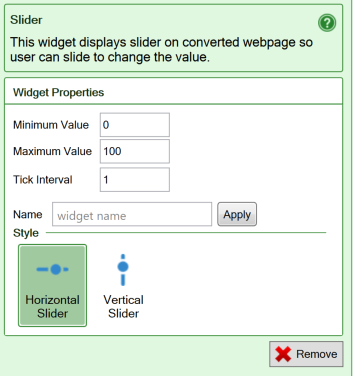
Learn more 
Some of our tutorials partly focus on the Slider widget:
Stepper 
The Stepper widget allows you to easily input small numeric values with just a tap or click on a button.
The worksheet is re-evaluated for each new value, making this a very useful widget when the user is trying to find an optimum value.

- The Minimum value is the lowest value the widget can have. The minus button stops working at the minimum value.
- The Maximum value is the highest value the widget can have. The plus button stops working at the maximum value.
- Use the Tick Interval if you want the step to be different from 1.
- Name your widgets if you want to pass data into them from the link to the form (see below). For electronic forms, it is also much easier to process the form if all input fields have names. You can name your fields in the widgets or give them cell names in Excel. Widget names can start with numbers or an underscore, which is required when integrating with products like Salesforce.
- The default value of a stepper is whatever value you put in the cell, or the minimum value.
- You can assign a value to a stepper widget from the link. Use the format /form.htm?example=2. Read more about filling form fields from the link.
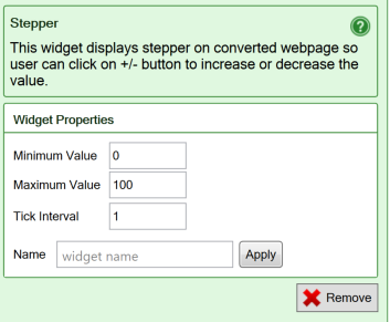
Rating 
Ratings widgets are used to rate, or grade, an experience or a product with symbols like stars. It’s an effective way of expressing one’s opinion about something.

You insert a Ratings widget by clicking the Ratings widget in the Widgets tab in the task pane.
- The Number of rating steps determines the number of stars in the widget.
- Name your widgets if you want to pass data into them from the link to the form (see below). For electronic forms, it is also much easier to process the form if all input fields have names. You can name your fields in the widgets or give them cell names in Excel. Widget names can start with numbers or an underscore, which is required when integrating with products like Salesforce.
- The default value of a rating widget is 0. To provide a different default value, enter an integer within the number of rating steps into the cell.
- You can assign a value to a rating widget from the link. Use the format /form.htm?example=4. Read more about filling form fields from the link.
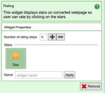
Calendar 
Calendar widgets make it much easier for the user to pick the right date. It also makes it easier to count from one date to another. The widgets ensure that any date picked from the calendar is valid, and formats it correctly for the recipient of the electronic web form using the regional settings.
Link Image 
Save all relevant image links in your spreadsheet or create formulas that can build the right image link dynamically from user input.
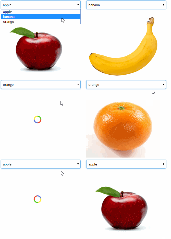
Use the Link Image widget to select the image that is shown.
Barcode widget 
Use the barcode widget to display a barcode from static or calculated content in your web form.
Check box 
Use check boxes only for statements that must be either true or false, there is no room for doubt, like “British citizen”. The Toggle switch allows you to use any two other names for True and False, e.g. a language pair.
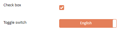
Touch checkbox 
You insert a Check box widget by clicking the Check box widget in the Widgets tab in the task pane. A Check box will provide a true/false value that you can test for in other places in the form, or when the form is submitted for processing.
- A Touch Checkbox looks like the check mark in the widget’s icon.
- When you add a Touch Checkbox to a spreadsheet, it is initially set to FALSE. When you convert the spreadsheet to a web page, a Touch Checkbox widget will therefore initially be unchecked. If you change the default value by typing TRUE into the widget’s spreadsheet cell before conversion, the Touch Checkbox will be checked when the page is opened in a web browser.
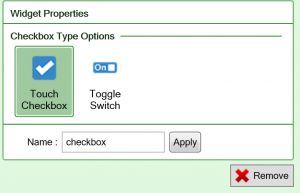
Toggle Switch checkbox 
- The Toggle Switch check-box is a small graphic that is intended to resemble an electric switch. Users can drag the handle or tap one side of the switch to toggle the check-box.
- When you flip the switch to the right, it returns a TRUE value. Flip it to the left and it sets a FALSE value for the cell.
- A Toggle Switch has two labels: one for each state. The On Label is visible in the switch when the value of the cell is TRUE and the switch is flipped to the right.
- Only the selected state is visible in the widget, e.g. Show. Your users will assume that flipping the switch will set the opposite state, e.g. Hide.
- When you add a Toggle Switch check-box to a spreadsheet, it is initially set to FALSE. When you convert the spreadsheet to a web page, a toggle switch will therefore initially show its Off Label, flipped to the left. If you change the default value by typing TRUE into the widget’s spreadsheet cell before conversion, the check-box will be flipped to the right and show its On Label when the page is opened in a web browser.
- Note: a cell containing a Toggle switch always returns TRUE or FALSE. It does not contain the text from the On Label or Off Label. If you need this function, use a Radio button instead.
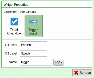
Common settings 
- Name your widgets if you want to pass data into them from the link to the form (see below). For electronic forms, it is also much easier to process the form if all input fields have names. You can name your fields in the widgets or give them cell names in Excel. Widget names can start with numbers or an underscore, which is required when integrating with products like Salesforce.
- You can set the value of a checkbox widget from the link. Use the format /form.htm?example=TRUE. Read more about filling form fields from the link.
Radio button 
Radio buttons simulate the behavior of old car radios. When one of the buttons is pressed, the corresponding radio station (option) is selected. Simultaneously, all the other buttons pop out, leaving only the selected button in the pushed-in position.

Radio buttons are used to select between a limited number of choices. The good thing about radio buttons is that you see all the available choices. The bad thing is that this may consume a lot of screen space. You insert a Radio buttons widget by clicking the Radio Button widget in the Widgets tab in the task pane. You can then set different properties for the Radio button widget:
- A Required field requires input from the user. This option is mainly used for electronic forms, where a form must contain a minimum of information to be meaningful. For Radio buttons, one of the buttons must be “pressed”. If no button is selected, it will not be possible to submit the form.
- Button labels are the names for each button. You get one button for each label you enter.
- In a Vertical Layout, the buttons are aligned in a column. Select the number of Columns to use for the choices.
- In a Horizontal Layout, the buttons are aligned in a row. Select the number of Rows to use for the choices.
- Name your widgets if you want to pass data into them from the link to the form (see below). For electronic forms, it is also much easier to process the form if all input fields have names. You can name your fields in the widgets or give them cell names in Excel. Widget names can start with numbers or an underscore, which is required when integrating with products like Salesforce.
- The default value of a radio button is the first choice on the list. To provide a different default value, move one of the other choices to the top of the list.
- You can select an option in the radio button from the link. Use the format /form.htm?example=Female. Read more about filling form fields from the link.
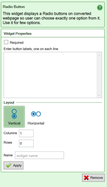
Dropdown 
Drop-down lists are used to select between a limited number of choices. The menu opens when you click on it. When you have made your choice, only the selected choice is visible.
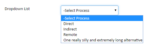
You insert a Dropdown list widget by clicking the Dropdown List widget in the Widgets tab in the task pane. List the labels in each line in the empty space. You can then set different properties for the Dropdown List:
- A Required field requires input from the user. This option is mainly used for electronic forms, where a form must contain a minimum of information to be meaningful. For Drop-down lists, the user must move the menu away from the option that is selected by default. If the default option is left selected, it will not be possible to submit the form.
- Show default text instructs the widget to add a dummy choice at the top of the list that implies that no “real” option has been selected yet – typically it’s is also used as a prompt, as in
“Rate the course, 4 is the best”. - List labels are the possible choices on the menu.
- Name your widgets if you want to pass data into them from the link to the form (see below). For electronic forms, it is also much easier to process the form if all input fields have names. You can name your fields in the widgets or give them cell names in Excel. Widget names can start with numbers or an underscore, which is required when integrating with products like Salesforce.
- The default value of a drop-down list is the first choice in the list. To provide a different default value, move one of the other choices to the top of the list.
- You can select an option in the dropdown widget from the link. Use the format /form.htm?example=Banana. Read more about filling form fields from the link.
- The basic Dropdown widget can only have one static list of choices. If you need a multi-level menu structure, e.g. select country then city, or want to prepare the list of choices with formulas in the spreadsheet, use the Dynamic Dropdown widget instead.
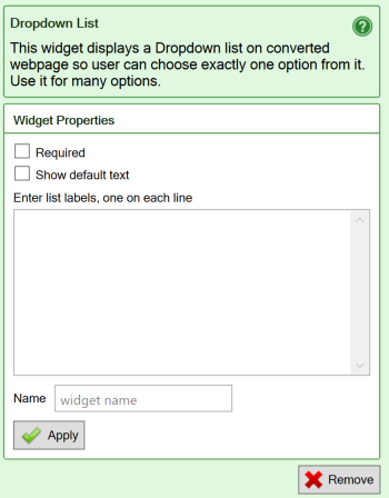
Dynamic Dropdown 
If you want the options in a dropdown menu taken from cells in the spreadsheet, learn more about the Dynamic Dropdown widget.
Hyperlink and Button 
The Hyperlink widget allows you to easily insert links into the converted web page, either as text links or as buttons.

Any cell in your worksheet can contain a web address in the form of a Universal Resource Locator or URL:
Unfortunately, Excel considers this to be just plain text. Nothing will happen if you click on this cell. If you convert this spreadsheet to a web page, the URL is generated as plain text there too, and clicking on it will have no effect.
To turn a URL into a working link, you have to insert a hyperlink into the cell. Excel can optionally create a hyperlink automatically every time you enter a URL into a cell, and then the link itself is used also as the anchor text for the link. To use any anchor text you like in the link, you can use the Insert Hyperlink command:
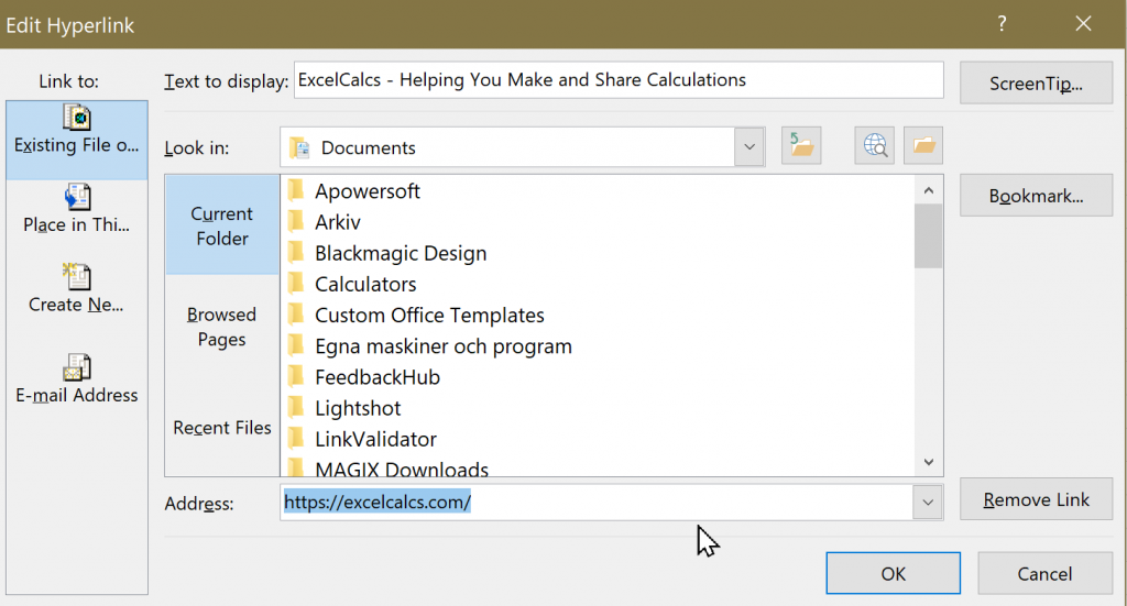
Notice that the anchor text, in the Text to display field, can be different from the link’s Address, when you use the Insert Hyperlink dialog to create the link. Users easily detect when a cell contains a hyperlink, because of its classic formatting in blue with an underline:

By default, SpreadsheetConverter preserves hyperlinks on the converted web page. The anchor text will be displayed and linked to the requested URL.
With Excel, a link can also be calculated with the
=HYPERLINK(Address, Text to display)
function. In this case, the Address portion of the link is assembled dynamically according to the formula you have specified. The URL may be determined conditionally using the IF function or the address assembled from other cells. The Address to use in a given situation can even be selected with the VLOOKUP function from a list of links. The Text to display operand of the Hyperlink function allows you to define the anchor text for the link.
=HYPERLINK("https://excelcalcs.com/","ExcelCalcs - Helping You Make and Share Calculations")
The Hyperlink widget provides a few additional useful features:
- A Style setting that allows you to present the link also as a button, either in the cell or in the toolbar. The link’s anchor text will be used on the button. The design of the button can be modified by a theme.
- A Placement setting where you specify if you want the link or button to be placed in the cell or in the toolbar.
- An Open In setting that lets you specify how you want the linked page to open: in the same browser tab, in a new browser tab, in the same frame of the web page or in the parent frameset. In the generated HTML, this selection is reflected in the HTML target parameter for the link, which will be omitted, set to _blank, set to _self or set to _parent, respectively.
- Name your widgets if you want to pass data into them from the link to the form (see the Text field widget above). For electronic forms, it is also much easier to process the form if all input fields have names. You can name your fields in the widgets or give them cell names in Excel. Widget names can start with numbers or an underscore, which is required when integrating with products like Salesforce.
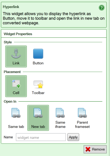
Email button 
An E-mail Button converts to a mailto (“send an e-mail to this e-mail address”) hyperlink. When the button is pressed, the default e-mail client normally opens a new, empty e-mail with the provided e-mail address as the e-mail recipient. The user enters the Subject and Text for the e-mail, then clicks Send to send the e-mail.
Note that none of this functionality is provided by SpreadsheetConverter. It is up to the user’s web browser to handle mailto links. If the user’s web browser is not properly configured to handle mailto links, the results are unpredictable.

The contents of your web form or calculator will not be involved in the processing started by the E-mail Button widget. If you wish to submit the full contents of a form or calculator, configure the web form’s submit options.
- Enter the recipient’s e-mail address in the Mail To field. The From field of the new e-mail will normally be set automatically by the e-mail client. All other fields of the new e-mail will be empty.
Call Button 
A Call Button converts to a tel (“initiate a telephone call to this number”) hyperlink. When the button is pressed, the device will initiate its normal behavior for tel hyperlinks, which usually is to make a telephone call to the number you have specified.
Note that none of this functionality is provided by SpreadsheetConverter. It is up to the user’s web browser to handle tel links. If the user’s web browser is not properly configured to handle tel links, the results are unpredictable.

The contents of your web form or calculator do not participate in the processing started by the Call Button widget, and nothing is sent to the designated telephone number.
- Enter the number you want the device to call in the Tel No field. The telephony infrastructure may require that you provide the phone number in a specific format. We recommend that you provide both country and area codes to ensure that the telephone number always works, regardless of the user’s location. The telephony infrastructure will usually also provide a Caller ID, i.e. the telephone number that the call originates from.
Action Buttons 
The Update, Reset, Print and Submit buttons are normally available in the toolbar.
If you want to place an action button elsewhere, perhaps to simplify the user interface, action buttons can be inserted as widgets in any cell in the calculator.
The text on the buttons can be changed. Just type the text you want on the button into the cell where you place the widget.
Submit Action button 
The Submit button sends the form to a web server for processing. Insert a Submit button at the end of your long form to save your users from having to scroll to the nearest toolbar.
Update Action button 
For smaller calculators, SpreadsheetConverter automatically updates all cells in a spreadsheet if one of the values is changed, just like Excel does. For a very complex web calculator, you have the option of switching to manual updating of the calculator in the Recalculation method setting on the Workbook tab. In that case, an Update button is needed to manually initiate the updating of the spreadsheet.
You can place the Update button in any cell, perhaps right after your most commonly used input fields.
Reset Action button 
The Reset button clears all input fields in a form. It is rarely implemented, except in situations where a large number of fields contain values that never will be re-used. You can make the Reset button available where-ever users need it.
Print action button 
SpreadsheetConverter supports three printing operations:
- Print All – prints all worksheets separately.
- Print This – prints the current worksheet.
- Print – prints the print sheet if there is one, or the current worksheet.
If you initiate the print operation from the web browser with the Print menu option or the Ctrl-P keyboard shortcut, it corresponds to the Print operation in the list above.
For each Print operation, there is an action button that you can insert into any cell in the spreadsheet.
Hide Rows/Sheets widget 
You can hide certain rows in your spreadsheet, and even entire worksheets, depending on the contents of a controlling cell.

Add/Edit Responsive Block widget 
Responsive blocks allow you to dynamically adapt the layout of the converted web page to the screen width of any device.

File Attachments widget 
If your users want to include files with their form submissions, e.g. a CV with a job application or an image with an error report, add a File Attachments widget to your form.
Utility 
The Utility widget can be used to assign a name to a calculated cell, or to make it invisible.
You insert a Utility widget by clicking the Utility widget in the Widgets tab in the task pane. Utility cells in a form or calculator are always locked for user input in order to preserve the contents.
- Make hidden field is used when you want a cell to be visible in the spreadsheet, but not in the converted web page. This also allows you to provide information to a form processing script without showing it in the form. As an example, if you use a cell to keep track of how long it took a user to fill in a form, you may want to hide this calculation. Even though the field is hidden, it is forwarded with the form when the form is submitted for processing.
- Name your widgets in electronic forms since it becomes much easier to process the form if all input fields have names. You can name your fields in the widgets or give them cell names in Excel. Widget names can start with numbers or an underscore, which is required when integrating with products like Salesforce.
- Utility cells get their default values from the formulas in the cell.
- You cannot assign a value to a Utility cell from the link to the web page.
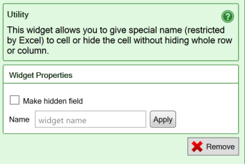
Learn more 
Some of our tutorials partly focus on the Utility widget:
Visitor and conversion tracking 
Visitor and conversion tracking 
Monitor the activity on your website using visitor and conversion tracking.
Visitor and conversion tracking 
When you create a calculating web page from an Excel spreadsheet, we can include scripts for visitor tracking. For conversion tracking, you use a thank-you page with an embedded tracking script.
SpreadsheetConverter has built-in support for visitor tracking using Google Universal Analytics. If you provide your Google Analytics Tracking ID, a standard tracking script will be inserted into each converted web page. Every subsequent visit to the calculator or web form will be tracked in your Google Analytics account. Read more in the first section below.
Conversion tracking is used to register special “success” events. With SpreadsheetConverter, such an event may be a validated form submission, e.g. a new user signs up for a mailing list. Insert the conversion tracking script into the thank-you page for the event. Activate the thank-you page for the web form in the Submit configuration. That’s it! When the thank-you page is opened in the user’s web browser after the form has been submitted, the tracking script in the thank-you page tracks the conversion. Read more about conversion tracking in the second section below.
Google Analytics visitor tracking 
When you convert a spreadsheet for the web with SpreadsheetConverter, you can automatically insert a Google Universal Analytics tracking script into the generated code.
To do this, enter your Google Analytics Tracking ID in the Workbook > Web page options section of the task pane.
The Google Analytics tracking code 
For each subsequent conversion, a Google Analytics universal tracking script for the provided tracking ID will automatically be inserted into the converted web pages.
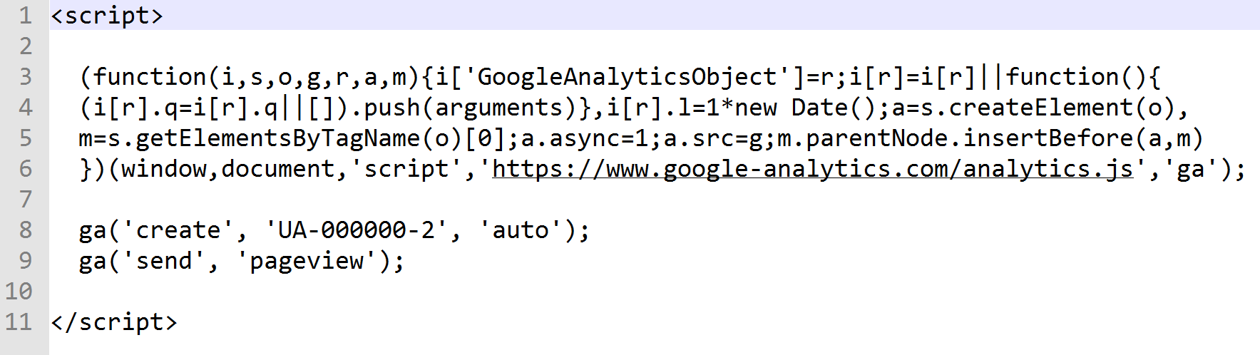
Finding the tracking code 
If you want to verify or modify the tracking code, it is inserted in .js files that are located in the output folder structure for the spreadsheet in the conversion path.
The default file system path to the conversion output is <username>/Documents/SpreadsheetConverter/. If you can’t find this folder, navigate to the SpreadsheetConverter ribbon menu in Excel, open the Options > Browsers and Conversion Path window and follow the Conversion Path setting to the conversion output folders.
Note: if you use OneDrive, there may also be a /Documents/ folder in the main OneDrive folder. Depending on your system settings, this folder may be used instead of the <username>/Documents/ folder.
In the conversion output folder, there is one folder for each spreadsheet you have converted. Inside this folder, you should enter the /public/ folder if there is one, then the /assets/js/ folder.
If Combine JS and CSS files is selected in Options > User Settings > Advanced Settings, the Google Analytics code is inserted into the app.min.js file. Otherwise, the Google Analytics code is inserted into the ssc.script.js file.
Using Google Analytics to verify the pageviews 
All visits to your calculating web pages and forms will be tracked in Google Analytics just like any other page on your website. You will find all visits to the page under Analytics > Behavior > Site content > All pages. In the example below we filtered the list for “/calculate/” since this is the folder where we store all our example calculators.
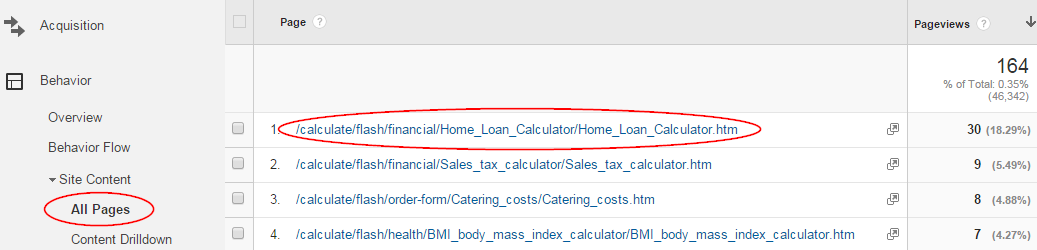
If your Google Analytics Tracking ID changes, or if you need to use more than one tracking ID, you must change the setting before you convert the affected web pages. The tracking ID for any web page you have already converted will remain the same as it was when the corresponding spreadsheet was last converted.
Other visitor tracking systems 
If you use another visitor tracking system, you need to manually insert a visitor tracking script for your tracking system into the HTML source for each converted web page.
If you intend to show the calculator in an iframe, or cut-and-paste the HTML source for the calculator into the source for an existing web page that already has visitor tracking enabled for it, there is no need to add a separate tracking script for the calculator.
Conversion tracking 
When your website receives visitors from advertising or external marketing partners, you may want to track a predefined “success” event, e.g.
- a confirmed sale
- a new user registration
- a validated survey response.
In web marketing, events like these are called conversions.
What you exactly choose to define as a conversion is up to you. It is one of the objectives, the goals that your website is trying to reach. A website usually has multiple goals. As an example, you could have goals like this:
- The user signs up for a newsletter.
- The user responds to a survey.
- The user buys a product.
The conversions count may be used for several different things. To improve the quality of pay-per-click advertising in search engines, you may want to study the conversion report from the search engine. The below example is from Google Ads and shows you the number of successful conversions per search term, and the average advertising cost to achieve a conversion for each search term. This information allows you to add more and more profitable search terms, and remove the unprofitable ones.
If you receive web visitors from other external sources, you can use an affiliate marketing system to track conversions and calculate the commission to pay each affiliate at the end of the month. In this case, a conversion tracking code snippet would be provided by the affiliate marketing system.
Validate the form before submission 
With SpreadsheetConverter, a conversion is often a validated form submission. It is an obvious event that can easily be identified and counted.
SpreadsheetConverter makes it easy for you to secure that qualifying form submissions are valid and complete, by providing tools in the spreadsheet such as:
- Extensive support for the built-in Excel Data validation features.
- Data entry widgets like dropdown menus force the user to select only between approved responses.
- Required fields force the user to provide mandatory information.
- Ordinary Excel formulas can be used to validate any data entered into the form.
Using these tools, it is easy to create a web form that cannot be submitted until it is valid and complete. You can even hide the Submit action button completely until you approve all the contents of the form.
Create the thank-you page 
A conversion event is normally tracked using a special “thank-you” page for the form. The thank-you page usually informs the website visitor that the web formhas been received for processing. As an example, have a look at our own default Success page.
When you have created the thank-you page, insert the conversion tracking script into its HTML source. The conversion tracking script is provided by the software that will track your conversions, typically a search engine advertising service like Google Ads, or by an affiliate marketing system.
Configure the submit operation 
Open the spreadsheet and navigate to Workbook > Configure Submit in the task pane. Enter the link to the thank-you page into the After successful submit field.

When a visitor arrives at the website, a cookie is usually created to link the new visitor session to the source – often a search engine advertisement or an affiliate link. When the tracking script in the thank-you page is run, it will verify the cookie, count the event and provide conversion statistics for your reports just like in the Google Ads report above. If you open the thank-you page without having set the session cookie first, e.g. from a search engine, most tracking systems will correctly ignore this and not register a conversion.
The Messages tab 
The Messages tab 
The Messages tab summarizes any issues that were encountered during the conversion of the spreadsheet to a web page.
After you have run a conversion, SpreadsheetConverter automatically shows the Messages tab in the task pane. The Messages tab alerts you with a red notification containing the number of messages that were issued.
The messages from the most recent conversion are saved with the spreadsheet and re-appear every time you open it. When you initiate a new conversion of the spreadsheet, any old messages are removed before the conversion starts.
There are three kinds of messages. Click on the corresponding button in the window to see the messages of each kind.
- Errors – the conversion did not end correctly.
- Warnings – These are things that will impact your use of the converted web page.
- Information – These are things you may want to know about.
Showing the full message text 
In the list of messages, click on the message you are interested in to see the full message text in the middle pane, and a list of affected cells in the bottom pane. To navigate to a particular cell, simply click the reference to the cell in the bottom pane and the cell will be selected.
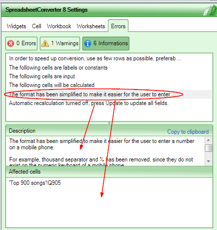
If an error or warning message was generated during conversion, your web page may generate incorrect results. You should always resolve such issues before using the page for calculations.
Below is a list of the most common messages and their meaning.
Informational messages 
The following cells are input
This message tells you what cells will be open for user input when the web page is opened in a browser. If a cell isn’t open for input when you expected it to be, read more about opening cells for user input.
The following cells are labels or constants
A label cell contains the label (caption) for a field, e.g. “Address:”. A constant cell contains a fixed value that cannot be changed. If the list contains a cell that you expected to become an input cell, read more about opening cells for user input.
The following cells will be calculated
A calculated cell is a cell that contains a formula. The converter uses this message to confirm that it has detected the formula and will calculate it automatically when the web page is modified in a web browser. If one or more cells are missing in this list, i.e. you expected them to be calculated but they were considered input or label cells, verify that the cell calculates correctly in the Excel environment. The equal sign may be missing, or there may be a separate error message for the formula in the cell.
Cells containing formulas cannot be input. Cell converted to output.
You have manually marked a cell as an input cell, but the cell contains a formula (beginning with “=”). Remove the formula from the cell or use another cell for input.
<Text format> does not work for in and out-cells.
Your spreadsheet uses a special text format for an input or output cell. Use a different format.
<Text format> not supported by HTML, using <text format> instead.
The former text format is not available for web pages and has been replaced by the latter text format.
Warning messages 
If you input dates, the format must follow <region> date format (<example>), since this is the standard format on this machine.
For input fields containing dates, the date format set in the Regional Options control panel must be used.
Overlapping ranges of different type (Num, Variant)
Error messages 
Dates containing name of month, weekdays or AM/PM cannot be entered using text fields. Choose 24-hour clock and dates like 01/02/2015.
Excel supports many date formats, including ones with the whole or partial names of months, e.g. “April 21, 2025”. These date formats are currently not supported for input fields. Use numerical date formats instead.
External file ‘file name’ referenced.
The converter requires that all worksheets required for the conversion are part of the same file. If you get this error message, one or more cells refer to an external file. If the cell that is referenced contains a static value, just copy it into a cell in the file you are converting and use the copied cell instead. If you need an entire worksheet from another file, copy the requested worksheet into the file you are converting and try again.
Error reporting 
If you get any error messages you don’t understand, we welcome you to contact our Help Desk. For your convenience, we have made it possible to report conversion errors and ask questions directly from the Messages tab in the task pane.
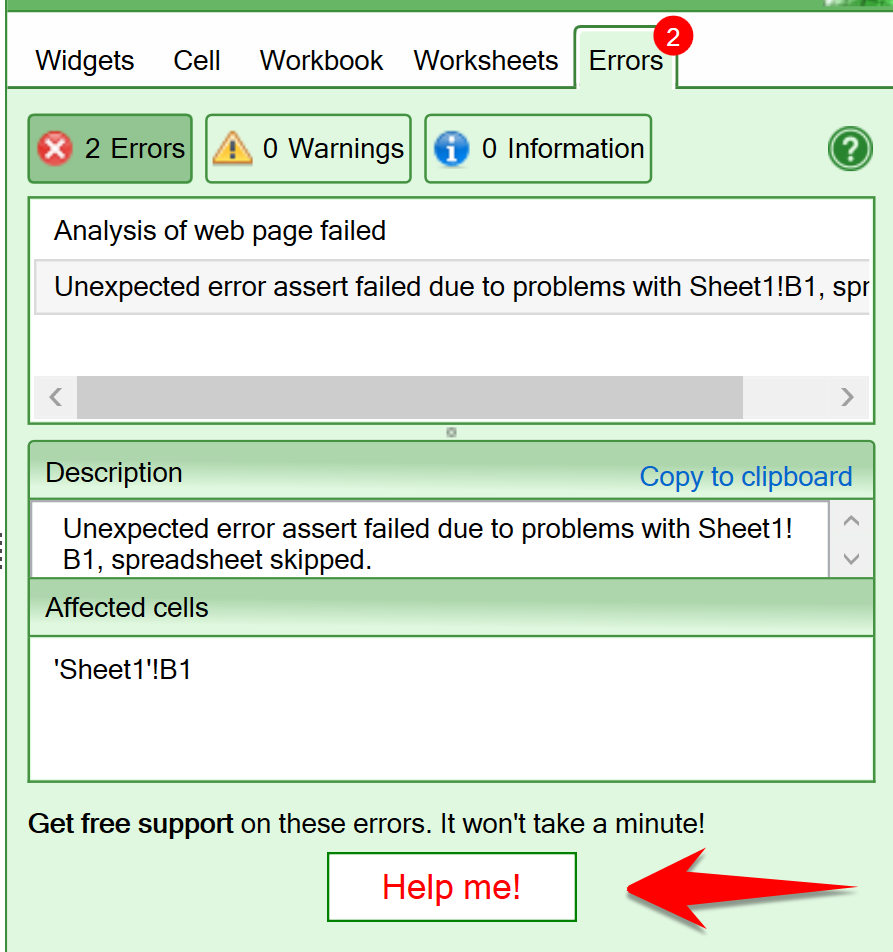
If you click the Help button, a form opens where you can enter your e-mail address and an error description. When you press Send the form is sent to our Help Desk.
When you submit the error report you can attach valuable debugging information depending on your choices in the Attachments section. Without some of this information, we may be unable to recreate many errors.
Help: Hide rows or sheets with a widget 
Hide Rows/Sheets widget 
Hide rows and entire worksheets in a form or calculator if a specific condition is true.
To make it easier to use an electronic form or calculator, you may want to hide certain rows in the spreadsheet until a specific condition is met. You may even want to hide entire worksheets unless other settings indicate that they are relevant.
To hide rows or worksheets in a spreadsheet, you can use the Hide Rows/Sheets widget. First, you specify what parts of the spreadsheet to hide, then you set the condition that will trigger the display of the selected rows or sheets.
Follow the step-by-step instructions below to use the Hide Rows/Sheets widget.
Example webpage: Hide Rows Sheet
Example spreadsheet: Hide_rows_sheets.xlsx
Insert the Hide Rows/Sheet widget 
Click on the Hide Rows Sheet icon in the Widgets tab of the task pane.
Click the Add new button.
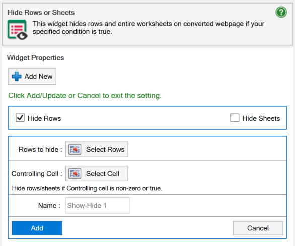
Select Hide Rows to hide rows and/or Hide Sheet to hide worksheets. If you select both options, the same controlling cell will hide both cells and worksheets.
For Hide Rows, an option named Rows to Hide will appear where you choose which rows to hide in the browser. Click on the Select Rows button and use the dialog box named Select Row range to select the range of rows to hide when a condition is true.
For Hide Sheets, an option named Sheet to hide will appear where you tick the checkbox for each sheet you want the browser to hide when a condition is true.
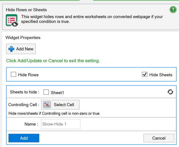
In the Controlling Cell option, select the cell which will control if the rows or worksheets are hidden or visible. If the value of the controlling cell is True or non-zero, the controlled rows and/or sheets are hidden.
The controlling cell may contain a checkbox widget, a textbox widget or any other widget that allows values to be entered.
An initial value for the controlling cell can be set from the link to the form or calculator. Read more in the next section.
To remember what this instance of the widget does, give it a descriptive name that tells you what you intended with the setup.
Press Add to activate the widget.
If you don’t want the controlling cell to be visible, insert a Utility Cell widget into the controlling cell and tick its option Make hidden field.
Convert the spreadsheet and test the form or calculator.
Use the link to the form to hide rows or sheets 
The value of the controlling cell can be assigned a value from the link, e.g. “../form.htm?hide_prices=true”.
The autosave process will normally save the latest value for all input fields in Browser Storage. This autosaved value will override the default value in the link. If hide_prices in the example above is unchecked on a form, it will appear as unchecked the next time the same user opens the same form. If you want the value in the link to override the autosaved value, you have to disable Browser Storage on the Workbook tab of the task pane.
Edit or remove the Hide Rows/Sheet widget. 
Click the Hide Rows/Sheet widget.
In the list of hidden rows/sheets, look for the name you provided earlier while hiding rows or sheets. If you want to edit the settings, click the name. If you want to remove the hide rows sheets instance, click on the Trash icon next to the name.
To edit a setting, click on the corresponding “pen” symbol.
The pen symbol beside the Rows to Hide option opens the Select Row range dialog box. Select the rows to hide in the worksheet if the condition is true.
The pen symbol beside the Controlling cell option opens the Select controlling cell dialog to let you select the cell which will make the worksheets or rows hidden or visible.
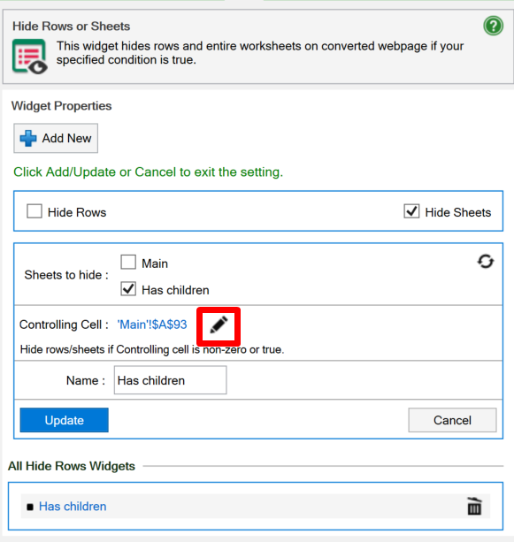
To change the sheets to hide, just check or uncheck the sheets accordingly.
Change the name of the widget instance, if required.
Click the Update button to save the updated settings.
Convert the spreadsheet and test the form or calculator.
Help: Introducing Responsive Design 
The advantages of responsive design 
SpreadsheetConverter supports industry-standard responsive web design, a methodology that automatically optimizes the layout of a web page for each screen. If you split your spreadsheet into logical blocks, these can flow nicely across screens of any size. With responsive design, your web pages look great and work well on any kind of device.
More and more web users have small devices with narrow screens. When you create web pages, you must ensure that these can be easily viewed also on mobile devices. Otherwise, your calculator may become difficult to understand or use for some of your most important visitors.
A responsive spreadsheet that adapts to the screen 

Historically, most spreadsheets were made very wide to fit the desktop screens of long ago. Today, this landscape-oriented design makes old spreadsheets difficult to use on smaller devices that are mostly used with the screen in portrait orientation. The unnecessarily wide layout requires a lot of horizontal scrolling.
With other development tools, you may be forced to create a separate “mobile” version of each spreadsheet. With SpreadsheetConverter you can instead easily divide the spreadsheet into responsive blocks that naturally flow across the screen to fit any screen width.
With responsive design, your web calculator or form automatically adapts to different screen widths.
- A visitor with a wide screen sees the responsive blocks for January, February and March in the same horizontal row.
- On a tablet, the calculator automatically shrinks to a two-column layout. The March block appears below the January and February blocks.
- On a phone, there is only room for a single block at a time on the narrow screen. The February block comes after the January block, before the March block.
Responsive blocks are easy to use and with little effort make almost any old and wide spreadsheet fit even the smallest screens.
Defining responsive blocks 

Maintaining separate versions of a spreadsheet for laptops, tablets and phones is time-consuming and complicated. With SpreadsheetConverter you can divide any Excel spreadsheet into Responsive Blocks of any size.
Each responsive block is a rectangular cell area that is always kept together, on all screens, regardless of the screen width.
The more width, the more blocks 
You define responsive blocks in Excel using the Responsive Blocks widget in the SpreadsheetConverter ribbon.
For each responsive block, you specify how much of the screen width to use for the block when it appears on the screen of a phone or tablet. If a block doesn’t fit to the right of the previous block, it appears at the beginning of the next row of blocks.
In the screenshot, you can see that the “AS” block requires the full screen width on a phone. On a tablet, however, it is only allocated half the screen width, so if the next block requires 50% or less of the screen width it will fit to the right of the “AS” block if the device is a tablet.
You can create fairly complicated layouts combining blocks of different widths, like
- 75% + 25%
- 50% + 33%
- 50% + 25% + 25%
and many other combinations. This lets you adapt the layout of your calculator dynamically to both phones and tablets without having to use separate designs for each device type.
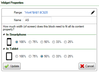
Preview your layout before you convert 
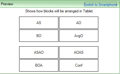

Does this sound complicated? Don’t worry. The Preview function is your best friend. After you’ve split your spreadsheet into responsive blocks, you can preview the automatic layout for both phone and tablet, and adjust your settings if necessary.
When the preview looks good it’s time to convert the spreadsheet for the web and study the results in a web browser.
You don’t need a tablet or phone to verify your responsive design. The layout is responsive already on your laptop and will automatically adapt to any change to the size of your browser window. Just resize the browser window and you will see how the responsive blocks automatically reposition themselves for the new window width.
When you convert the spreadsheet to a web page, your calculator or form uses the responsive blocks to adapt itself to any visitor’s screen in the way that you have defined. Your calculating webpage automatically fits every screen size without horizontal scrolling.
Learn how to edit or delete responsive blocks
Before you create your first responsive spreadsheet, we suggest you read our best practices for responsive blocks to avoid the most common mistakes.
Help: Split web forms into two or more sections 
Some forms are so long or complicated that they need to be split into two or more separate sections. SpreadsheetConverter provides several different ways to work with such forms.
SpreadsheetConverter has many different ways to handle multi-sheet workbooks:
- Listview shows the sheet names in a list, and you click on a name to view a sheet. (Available in the iPhone/Android flavor only.)
- Tabs generates a tab for each worksheet in the workbook, much like Excel itself does, to let you select what sheet you want to work with. (Available in all flavors except iPhone/Android.)
- Wizard uses Next and Previous buttons in the toolbar to guide the user through a sequential step-by-step data entry process.
- Panels are horizontal headers, each representing a worksheet. When you click on a panel, the corresponding worksheet slides down to appear below it. If you click on the panel again, the worksheet disappears again by sliding in under the panel.
- Accordion layouts are similar to panel layouts but show only one section of the form at a time.
Make all required worksheets visible 
To work with more than one worksheet in a workbook, you must first make all the required worksheets visible in the converted web page. Hiding worksheets is done in the Worksheets tab in the task pane.
By default, SpreadsheetConverter shows only the active worksheet. If your spreadsheet contains more than one worksheet, click to make the “eye” symbol green to make the corresponding worksheets visible in the converted web page.
Listview layouts 
The Listview layout is only used for small screens when converting with the iPhone/Android flavor, and contains a list of the worksheets on the web page. The user scrolls to a sheet and clicks on it to view it. Any worksheet can be viewed at any time.

If the workbook is used as a multi-section form, it can be submitted for processing by pressing the Submit button on the Side menu.
Tabbed workbook layouts 
With a Tabs layout, SpreadsheetConverter generates a row of links at the top of the web page, with one link for each worksheet. Clicking on the Delivery or Billing link below takes you to the corresponding worksheet. The user can view any worksheet at any time.

If the workbook is used as a multi-section form, it can be submitted for processing by pressing the Submit button in the toolbar.
Data entry wizard layouts 
Choosing a wizard layout creates a sequential data entry wizard to guide the user through the various sections of the form. The user advances from each section to the next using a Next button.
The Previous button returns to preceding section of the form. Finish bypasses all remaining steps and immediately submits the form.
You can add a Cancel button that allows the user to exit from the wizard without submitting the form. To add a Cancel button, specify an URL for After Cancel in the wizard in the Workbook > Configure Submit settings.
All the button names can be modified in Preferences > Customize Texts.
So-called breadcrumbs appear at the bottom of the toolbar to give users a way to keep track of their location within the wizard (the term comes from the trail of breadcrumbs left by Hansel and Gretel in the popular fairytale).
Panel layouts 
Panels enable the user to view one or more worksheets simultaneously. The user can switch between sections of the form at will, or work with two or more sections at the same time.
In the example below, both the Products and Billing worksheets are visible at the same time.
A form created with panels can be submitted at any time by pressing the Submit button.
Accordion layouts 
With an accordion layout, only one section of the form is visible while the rest of the form is hidden. Clicking on the Products panel displays the Products worksheet.
Clicking on the Delivery panel closes the Products panel and opens the Delivery worksheet.
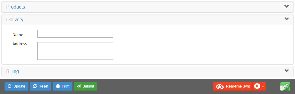
Forms created with an accordion layout are submitted with the Submit button.
Help: Follow us in the Notification center 
Notification Center 
The Notification Center keeps you up-to-date with the development of SpreadsheetConverter.
The Notification Center gives you information about product updates, new features etc so that you can keep up-to-date with SpreadsheetConverter. If you follow us in other ways, you can turn the Notification Center off.
Imagine that you just spent fifteen hours trying to solve a problem that has a better solution in the next version of SpreadsheetConverter – dull, hey? The Notification Center automatically informs you about new features, program releases, tips and tricks from the SpreadsheetConverter server. This helps you understand what you are missing in your current installation.
Here is an example of a live banner giving you a message about SpreadsheetConverter.
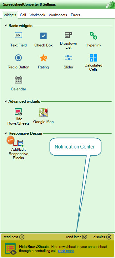
The way you use the Notification Center is simple:
- Read next: Moves on to the next message.
- Read later: Hides the live banner temporarily. It reappears the next time you start Excel.
- Dismiss: Hides the Notification Center permanently. To make the Notification Center visible again, reactivate it in Preferences > Show Notification Center in Task pane.
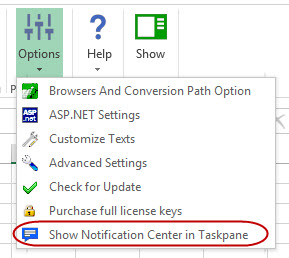
Help: Open cells for user input 
When spreadsheets are converted to web pages, all cells are locked for input except those required to use the form or calculator. For forms, you may want to unlock additional fields for input, e.g. text fields that aren’t used in any calculations.
SpreadsheetConverter makes a clear distinction between these types of cells:
- Cells that are open for user input are called input cells.
- Calculated cells that contain formulas are called output cells.
- Cells that contain text are called label cells.
- Empty cells are not open for input by default.
SpreadsheetConverter can automatically guess what cells in your worksheet you want to open for user input on the converted web page. It does this by looking at your formulas and seeing what cells they take their input values from.
If you want to use an empty cell for user input, or a cell containing text, you must explicitly open the cell for user input. There are several convenient ways to do this:
- automatic detection of input cells
- using widgets to open cells for input
- using a special background color for input cells
- unlocked cells are input cells
The settings for input cell designation 
The settings for input cell selection are on the Workbook tab in the task pane.
Switch to the SpreadsheetConverter ribbon 
In Excel, look for the SpreadsheetConverter tab at the right end of the menu ribbon. Click the tab to switch to the SpreadsheetConverter ribbon.
Open the Workbook tab 
In the SpreadsheetConverter ribbon, click on Workbook so that the SpreadsheetConverter task pane becomes visible.
Workbook > Input cells 
On the Workbook tab in the task pane, locate the Input Cells settings.
Automatic detection of input cells 
The first time you convert a particular spreadsheet, try using automatic detection first. Select Auto as the selection method.
With automatic detection, cell types are assigned like this:
- A cell that contains a Text widget becomes open for user input.
- A cell that contains a formula always becomes an output cell since allowing user input would overwrite the formula.
- An empty cell that is referenced by a formula is opened for user input. Example: If A1 is empty and B1 contains =A1+1 then A1 will become an input cell by default since the formula appears to require user input, and B1 becomes an output cell to protect the formula.
Using widgets to open cells for input 
Some input cells may not be obvious to SpreadsheetConverter’s automatic detection. If you are designing a form, you may want certain cells in the form to contain plain text input, e.g. address fields that you just want to be forwarded with the form when it is submitted.
All input widgets explicitly open cells for input, e.g:
- If you insert a Text widget into an empty cell, it is automatically opened for input on the web page.
- If you insert a Calendar widget, the cell automatically becomes an input cell.
- If you insert a Dynamic Dropdown widget into a cell, it is automatically unlocked for user input.
Using a special background color for input cells 
If you need to open a large cell range in the spreadsheet for input, it may be tedious to insert many Text widgets. In this case, it’s much quicker to use a special background cell color for the cells you want to open for input from the user. During conversion, SpreadsheetConverter locks all cells except the cells with the selected background color.
Begin by giving all input cells in the spreadsheet the same background color, in this example yellow. Ensure that you use a background color that is not used elsewhere in the workbook. You must background color all input cells, also the ones referenced by your formulas, since they will not be opened automatically.
Before conversion, select Cell color for Input Cells selection on the Workbook tab. Then click on one of the cells that have the selected background color.
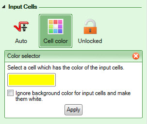
If you don’t want the input cells to actually use this background color on the web page, check the checkbox Ignore background color for input cells and make them white. You will still see the assigned color in Excel, but in the web page, all the input fields will have a white background.
Unlocked cells are input cells 
If your spreadsheet uses Excel’s built-in protection mechanism for locked cells, you can also use it to explicitly unlock input cells. You must unlock all input cells, also the ones referenced by your formulas, since they will not be opened automatically.
Select Unlocked for Input Cells selection on the Workbook tab. Remember to unlock the worksheet before conversion!
Learn more 
Some of our tutorials partly focus on opening cells for input:
Help: Scanning QR codes 
Quick Response Codes are easy to use. Just point your camera at the code and the corresponding web page opens in the web browser.
Quick Response Codes were developed in 1994 by Toyota’s subsidiary Denso Wave to allow automotive components to be scanned at high speed. QR Codes provide an easy way to print machine-readable information on paper. In its most compressed form, a single QR code contains several thousand characters.

QR codes have recently become popular also as a simple means to feed information into mobile devices, usually web addresses, from newspapers, subway advertisements or museum displays. If you use the standard camera app it will automatically open the related web page in the web browser. Many apps can also read and decode the QR Code through the camera, e.g. to fill form fields.
What you need 
Before you continue, consider the following:
- Your device must have a working camera.
- Your device must have an Internet connection at the time you scan the QR Code, to be able to open the web page.
- Modern smartphones can decode QR codes with the normal Camera app. Just point the camera at the code. In most cases, you will be prompted if you want to open the link in the code. For step-by-step instructions, read more below. On laptops and older phones, you may need a separate app to scan QR codes.
Installing a QR Code app 
If you have an older device or have disabled automatic QR Code scanning for the Camera app, you may need to install a separate QR Code scanner app on your device.
Beware that QR Codes can be malicious. Since they are impossible to decode with the human eye, there is no way for you to determine if the web page that will open in your device is the one you expect, or if it’s safe. We recommend scanners with built-in web security checks, e.g. Kaspersky QR Scanner or QR Pal from QR Pay Ltd, both available both for iOS and Android devices.
Visit the appropriate app store and download one of the many alternatives.
Scanning the QR Code 
- Start your Camera app (or a separate QR Code scanning app) and wait for the camera to power up. If your device has more than one camera, e.g. front and back, ensure you’ve selected the back camera so that you can focus the camera on the barcode using the display on the front.
- Point the camera at the QR Code. When your display shows the image from the camera, try to get as close to the screen as you can. You should be able to see how the camera automatically adjusts its focus and scans the code. The QR Code is automatically corrected for reading errors, so it’s unlikely that you will get an incorrect reading. You can scan the code with the phone in portrait or landscape mode; it doesn’t matter.
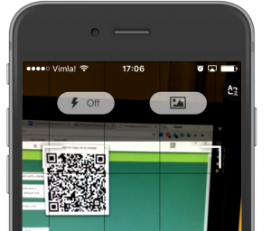
- Verify that the link points to the correct website. When the app has decoded the QR Code, the link is usually displayed on the screen. Some QR Code readers decipher shortened URLs (beginning with domain names like bit.ly, ow.ly or goo.gl), which makes it easier for you to verify the true destination address. QR Code readers with reputation control will also give you a report on the reputation of the site you will be visiting. If your barcode scanning app doesn’t have these features you may open a malicious website unless you verify the link carefully.
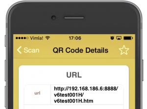
- Approve the decoded link if you feel secure that the address you just scanned is safe. This should open the web page from the QR code in your smartphone’s default web browser.
Using QR codes with laptops 
Many laptops have built-in cameras above their screens to facilitate video conference calls. Such web cameras can also be used to scan barcodes from another computer’s screen to open a particular web page on the laptop.
The easiest way to scan a barcode from a computer screen with a laptop is to hold the laptop upside down with the camera pointing at the barcode image on the other screen. It doesn’t matter that the QR code is read upside-down.
You only need to scan the code once 
If you are viewing a converted web page from another device, you only need to scan the barcode the first time you open the page. If the web page is already open on your mobile device, just press the Reload button. It is usually a circular arrow (it looks like a “rotate clockwise” symbol) and it is often located near the website address field.
On a phone, it can look like this:
On your laptop, it looks almost the same:

Help: Configure a web form's submit options 
SpreadsheetConverter automatically sends submitted web forms to any Inbox. The basic service is free. You enter the e-mail address in the Configure Submit options on the Workbook tab in the task pane.
You can build web forms that automatically get sent to your e-mail Inbox every time someone uses the form. For a small monthly fee, you can also have each submitted form stored in a hosted database for later retrieval. Read more about our Free and Advanced Submit Services.
When you create a web form, you need to specify to which e-mail address each submitted form is to be sent. There are also many other powerful options that let you tailor the forms submission process to your requirements.
Position the toolbar 
Select the action buttons for the toolbar 

The toolbar can include a number of different action buttons. The most important one is Submit since this is the button that is used to send a completed form for processing. This checkbox must be checked for every electronic form.
Open the Configure Submit window 

At the top of the Workbook settings, there is a button for configuration of the forms submission process, i.e. how completed forms should be forwarded for processing. Click on the button to open the Configure Submit window.
Enter the e-mail address that receives the forms 

Enter the e-mail address to which you want completed forms to be sent.
If you just want a one-time demonstration of what an e-mail from the Advanced submit service looks like, select Demonstration. Instead of being sent to your Inbox, a copy of the e-mail will open directly in your web browser every time you submit a new form.
Select the Advanced submit service if you have a trial or paid license for it, or select the Free submit service that is included with your SpreadsheetConverter license. The main difference between the two is that the Advanced service stores each form in a database, and formats the e-mail you get for each form submission exactly like the web form, which makes processing the form a lot easier.
Secure delivery 
If you have a license for the Advanced service, select the Secure Delivery option if you want the e-mail to contain just a link to the received form. This protects the form contents and any file attachments behind an additional login, making the e-mail you receive for the form look like this:
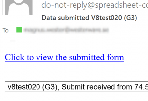
We recommend that you always use Secure Delivery if you allow file attachments for the form. Otherwise, file attachments are included in the e-mail with the completed form, which may cause problems if the files are very large.
“After submit” links 
After a form has been submitted, a “Thank you” window is displayed. Like all other standard texts, you can change or translate the text in this window using the Configure Text setting described above.
If you want to provide a full thank-you-page of your own, e.g. to provide conversion tracking, enter its address in the After successful submit field. Click the button to the right of this field to verify that the address is correct; if it is, the page will open in your web browser.
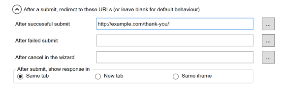
You can also provide your own handling of submissions where our server failed to receive or e-mail you the data. This can only happen when our server is stopped for some reason. The After failed submit link should point to a page that recommends the user to wait for ten minutes and then try again.
If a data entry wizard layout is used for a multi-sheet workbook, you can provide a Cancel button in the wizard that allows the user to leave the form without submitting it. In the After cancel in the wizard field, enter the address of the web page you want the user to arrive at after having pressed Cancel, e.g. a page where you attempt to convince the user to complete the survey anyway.
Use a better subject in the e-mail for each form 
When forms are submitted, you will get one e-mail for each form. These e-mails will have a standard subject line, identifying each form with a sequence number.
In many cases, it is much easier to find the right form among all the e-mails if you provide a better visual identification for the form, e.g.
- the customer’s name
- the city
- and the street address.
To accomplish this you must first prepare the entire subject line you wish to use for each e-mail in a separate cell in the spreadsheet, using a formula like this:
=cust_name & " " & cust_city & " " & cust_street1
E-mail subject lines don’t have to be unique in any way, so it’s no problem if there will be several forms with the same subject. A customized subject line is probably much more useful than our standard sequence number anyway.
Assuming you have put the above formula in cell A8 of the spreadsheet, you can now use the Manage the email subject line setting to replace the standard e-mail subject with your own. Just click on the Select Cell button, then select cell A8 in Excel.
When you’re done, it will look something like this:

There is also a shorthand notation: just give cell A8 the reserved name subject to assign the same setting.
Send the form to additional recipients, e.g. the submitter 
By default, each submitted form is sent to the Form Recipient, i.e. the e-mail address you entered into the Configure Submit settings above.
You can also send a copy of the submitted form to the person submitting the form – we call this the Form Submitter – or to any other e-mail address available in the spreadsheet. All you need to do is to designate a cell in the spreadsheet where the user is required to enter a valid e-mail address, and a copy of the submitted form will be sent also to the e-mail address in this field.
We recommend that you always use the Email widget for e-mail address fields since it automatically validates the syntax of the address and can make the field mandatory. As an example, if the submitter’s e-mail address is in cell A7 of the spreadsheet, you can now use this in the Send copy of email of submitted form to the submitter setting to provide an additional e-mail address. Just click on the Select Cell button, then select cell A7 in Excel.
When you’re done, it will look something like this:
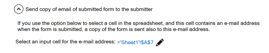
There is also a shorthand notation: just give cell A7 the reserved name email to assign the same setting.
Sending e-mails between Form Submitter and Form Recipient 
When a form contains an email field, it becomes easy for the person that submitted the form to communicate with the recipient, and vice versa.
- If the Form Recipient replies to the received form, the reply is sent to the Form Submitter e-mail address. This makes it easy for the recipient to follow-up on form submissions and ask additional questions.
- If the Form Submitter replies to the e-mail with the submitted form, this response is sent to the Form Recipient. This makes it easy for the submitter to provide additional information.
Use your own script for SpreadsheetConverter forms 
If you prefer to use your own script to process each submitted web form, enter a link to that script in the URL field.

If a worksheet contains two input fields, “cust_name” and “cust_city”, the values in these two fields are appended to the link to your script, making it look like this:
http://example.com/sscform.php?xl_version=16.0.0&cust_name=Microsoft%20Corp&cust_city=Seattle
Data is encoded according to the HTTP Post standards, e.g. a space is represented as “%20”. Please contact our support department if you need help on how to decode the query string of an HTTP Post operation.
The following parameters will be available to your script in the query string:
- xl_version=16.0.0 – identifies the file format
- (name1)=(value1) where (name1) is the name assigned to the first input cell in the form and (value1) is the content of that cell
- (name2)=(value2) the name and content of the second input field in the form
- etc
Only the form fields that are open for input are sent to the script. If there are 22 input fields in a form, there will be 22 name-value-pairs in the query string of the link to your script, plus one for the xl_version.
If you intend to use this feature, you should assign names to all the input cells in the form. Otherwise, SpreadsheetConverter has to refer to cells with an internal Excel coding that is based on the rows and columns of the original spreadsheet. Please contact our support department if you need help decoding this format.
Translating the messages from submit 
When a user presses the Submit button, all the form field are validated against the rules set for them, either in widget definitions or using Excel’s Data Validation. If one or more fields don’t pass this validation, they will get a red border and a message is issued. This message can be translated in the User Settings > Customize Text.
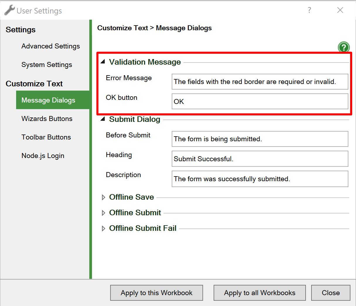
When the submit is valid, a message box will say that the new form is being queued for processing and then confirms that the submit operation was successful. These messages can also be translated in the User Settings > Customize Text.
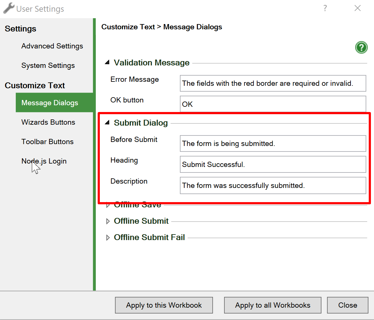
The text for the Submit button itself can be translated. If your form uses a standalone Submit button in a cell, it will get its text from the cell itself.
If the Submit button is in the toolbar, the text for this and the other buttons can be translated in the User Settings > Toolbar Buttons.
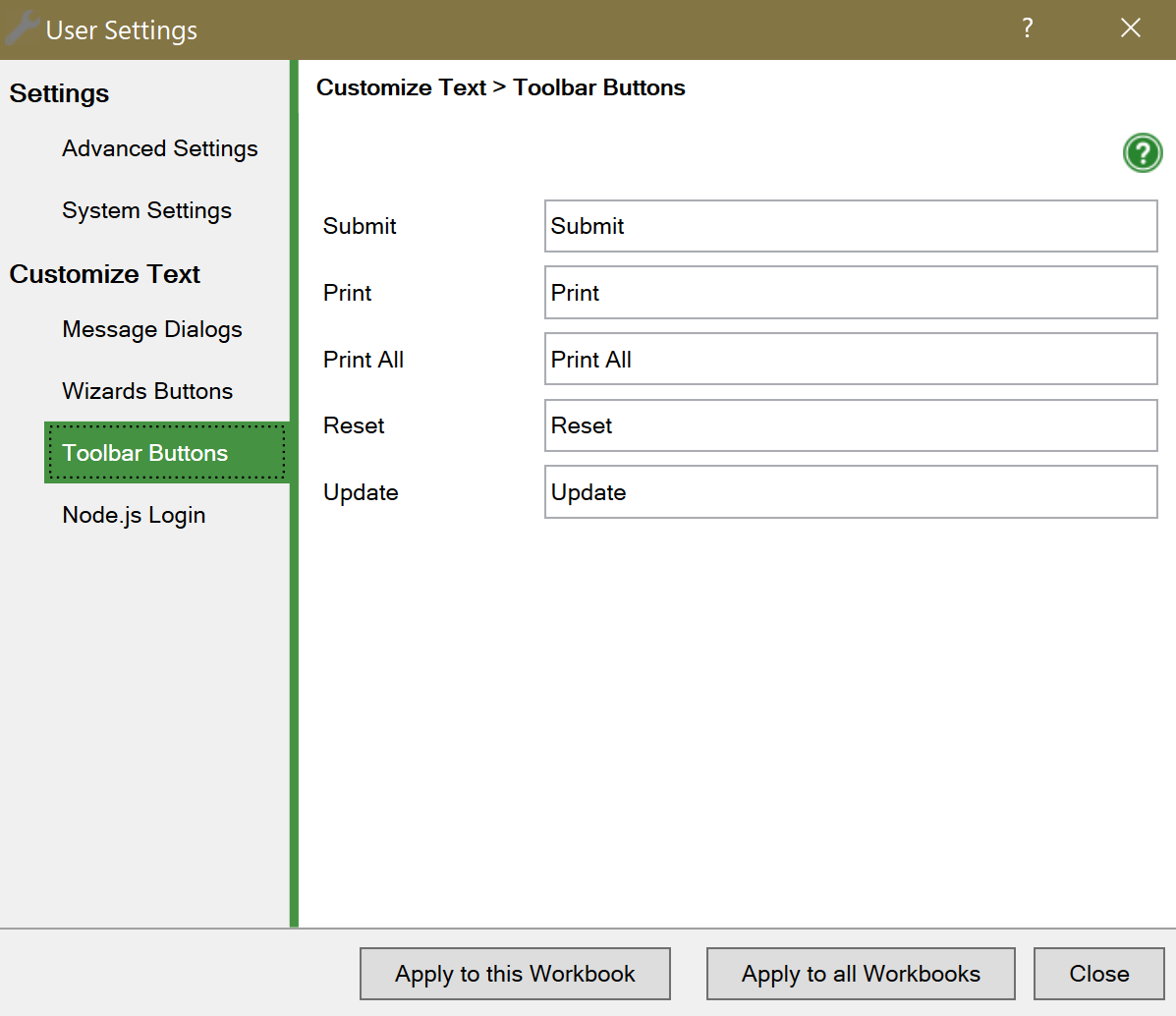
Special functions 
Our form solutions provide lots of added value:
- You can lock or hide form fields.
- You can make form fields mandatory.
- You can validate most common field formats like dates, numbers and e-mail addresses.
- All named cells can be pre-filled from the link to the form, e.g. /form.htm?email=x@y.z&subject=Application.
Read more in the tips and tricks section.
Learn more 
Some of our tutorials partly focus on the Configure Submit settings:
Known issues 
Sending electronic forms from a web browser to a web server and then on to an e-mail client has a few known issues.
Try this Excel add-in now! 



Click on Download to install and test this Excel add-in for Windows.
Click on Upload to let us convert a spreadsheet for you for free.
Help: Convert to Node.js flavor 
Converting for Node.js 
Step-by-step guide to converting your spreadsheet for Node.js and publishing it.
The Node.js flavor of SpreadsheetConverter builds secure server-side calculators for Node.js servers in which all your formulas are protected from copying and downloading.
To provide a secure operating environment for business-critical calculations, the new Node.js flavor of SpreadsheetConverter creates the program code separately from the web page. When a website visitor wants to use the calculator, the web browser downloads the web page from the web server without any sensitive program code. Instead, special code snippets in the web page act as conduits between the web page and the program code on the Node.js server. This effectively hides the spreadsheet’s formulas and their program counterparts from any prying eyes.
Learn more about the difference between client- and server-based calculation.
Tutorial 
The below tutorial will show you how to convert a spreadsheet into a Node.js web calculator and publish it.
Please follow the steps below.
Start Excel 
Start Excel and verify that the SpreadsheetConverter ribbon is visible in the menu bar. If it isn’t, make sure that SpreadsheetConverter is properly installed before you continue.
Also check that the Node.js flavor is visible in the Conversion menu in the SpreadsheetConverter ribbon. If it is not, your free trial period may have expired and you need to purchase a license for Node.js before you continue.
Open the spreadsheet 
Open your spreadsheet in Excel.
Select the Node.js flavor 
Select the Node.js flavor in the ribbon.

Convert the spreadsheet 
Press the “Convert” button.

Verify the result 
Just like with the other flavors, the converted Node.js application will be automatically opened in one or more of your web browsers, depending on your settings.
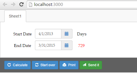
Technical note: Since Node.js is a server environment, a bit of extra magic is required to open the converted web page, including starting a miniature web server that runs the Node.js environment in your Windows system. If you restart your computer, this setup will be discarded automatically and the localhost URL won’t work any longer. To view the web page after a restart you just convert the spreadsheet again.
Publish the page on the web 
You can test your Node.js calculator using our Test in Cloud service. Your just converted Node.js application is uploaded to one of our Node.js hosting servers for testing. The test link is valid for seven days.
Learn more on the help page for Test in Cloud.
Upload the web page to your Node.js environment 
After testing you should upload the Node.js calculator to its production environment. This can be Node.js running on one of your own servers. You can also use any third-party Node.js hosting provider.
A word of caution: many Node.js hosting providers require a bit of experience with Command-line and Git. Some hosting providers like EvenNode let you use FTP instead of GIT.
Autosave form fields in browser storage 
Autosave form fields in browser storage 
Everything you type into a form is automatically saved. In case of a system or network error, you can always return to where you were. If you want to use your standard contact information over and over again, you don’t have to do anything – it is already there the next time you open the form.
Having to re-enter all the values in a web form every time you open it can be very painful, and even frustrating when dealing with large forms with numerous input fields. Usually, your users want to retain a lot of the contents from the previous form.
Whenever an electronic form is open in a web browser, we automatically save the content of all the form fields. If the same form is opened again later, the field contents from the last visit are re-used.
This gives several advantages:
- It’s easier to fill in multiple forms where some information like contact fields have the same content every time.
- All form contents survive system errors, unexpected restarts and network errors. When everything is back to normal, just open the form again and you are back where you left it.
The autosave functionality is automatically enabled when you Enable Browser storage on the Workbook tab.
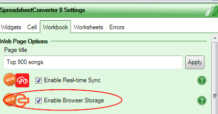
Browser Storage 
Browser Storage 
Browser storage, provided by the user’s web browser, allows us to re-use the most recent field values. If the user is offline, we can also save forms offline until the user comes online again.
As a service to your users, we pre-fill each web form they open with the most recent values they used for the same form.
Using Browser Storage we can store at least 150,000 input fields, well enough for any form we expect anyone to build with SpreadsheetConverter. This allows you to create forms as big as you like and still save your users a lot of time by having their most recent input values automatically retained.
Browser storage is provided by all modern web browsers. It is similar to the Luggage room in most major hotels – just like you can put your suitcase in the Luggage room on your first or last day at the hotel, web browsers allow us to save data in their “Luggage room”, and we can come back whenever we like and pick it up. If we don’t, it can stay there forever.
Auto save vs defaults in the link 
A good thing is that you can provide a default value for most named form fields in the link to the form, e.g. /form.htm?lang=sv. Learn more about filling form fields from the link.
Another good thing is that whenever an electronic form is open in a web browser, we automatically save the content of all the form fields. If the same form is opened again later, the field contents from the last visit are re-used. Read more about autosaving form fields.
What could be a problem, however, is that the autosaved values from the previous form always override any default values in the link. If you want the values in the link to override the autosaved values from the previous form, you have to disable form field autosave. You do this by disabling Browser Storage on the Workbook tab according to the instructions below.
Disable Browser storage 
Browser storage is enabled by default for all web pages you create with SpreadsheetConverter. If you wish to disable Browser storage, uncheck the Enable Browser Storage setting on the Workbook tab of the task pane. When you convert a spreadsheet again, the new setting will be used for the converted web page.
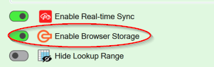

The Browser Storage Toolbar 
If users complain that their web forms open with garbled data, it may be the result of a previous error that was then saved with the rest of the field contents in Browser Storage. The easiest way to clear a form from previous field contents is to press the Reset button. This should restore the original, default values in all input fields. If this doesn’t help, there is the heavy artillery – the Browser Storage Toolbar.
For the Browser Storage Toolbar to appear for a converted web page, you must convert the spreadsheet with the Enable Debug Mode Conversion setting. This setting is located in the Ribbon > Options > User Settings > Advanced settings.
Remember to turn the setting off after you’ve converted the spreadsheet, otherwise it will activate the Debug Mode for all subsequent conversions.
When you open a web page in Debug Mode in Firefox or Internet Explorer, the Browser Storage Toolbar appears at the bottom of the screen.

Press the two blue buttons to have the current use of Browser Storage calculated.

The two red buttons allow you delete any Offline Submits (saved forms and e-mail templates) or all Browser Storage (including saved field contents). Despite the icon, there is no recycle bin here – deleted is deleted.
Using the Browser Storage Toolbar can help you and your form users get out of most problems related to saving previous field contents in Browser Storage.
Embed a Live Spreadsheet in WordPress 
Embed a Live Spreadsheet in WordPress 
When you convert an Excel spreadsheet to web format and upload it to WordPress you can embed it in one or more web pages and it will work like in Excel.
Before you embed a spreadsheet in WordPress you convert it to web format with SpreadsheetConverter. Then you use a special plugin in WordPress to upload the SSC Calculator file you get as a result of the conversion. If you haven’t yet converted the spreadsheet or uploaded it to WordPress you need to start over from the beginning.
Now, it’s time to embed the calculator in one or more web pages. The steps are a little different, depending on what WordPress editor you are using.
Embed a spreadsheet with the Block editor 
In WordPress, click on the Upload SSC Calculator link in the menu.
In the list of calculators, locate the calculator you want to embed. In the column Calculator iframe, click on the Click to Copy button for the calculator you want to embed. This copies the complete embed code to the clipboard.
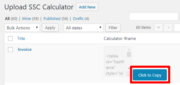
Open the Block editor for the page or post where you want the uploaded calculator to appear.
Click on the plus sign to insert a new block. Type “html” in the search box and select to insert a Custom HTML block. To move the Custom HTML block to the correct position on the page, drag it using the handle on the left-hand side or use the up/down arrows.
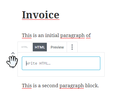
Select the HTML view for the Custom HTML block. Paste the embed code HTML into the Custom HTML block with Ctrl+V or right mouseclick+Paste.
Select the Preview view for the block.
Remove the toolbar 
By default, SpreadsheetConverter adds a toolbar at the bottom of the online spreadsheet. If you want to remove the toolbar, follow the instructions at the bottom of this page.
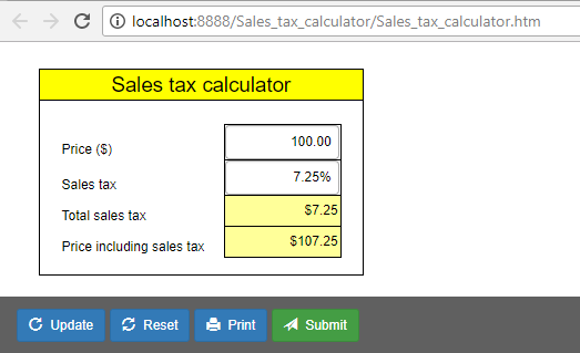
Change the size of the calculator on the page 
If you cannot see the entire calculator, or if scrollbars appear, or if there’s too much whitespace around the calculator, you may need to adjust the size of the iframe. Select the HTML view for the Custom HTML block, adjust the height and width parameters in the <table id=”hasIframe” tag that represents the calculator, switching back and forth to the Preview tab until the calculator looks good. Don’t be afraid of leaving a considerable margin around the calculator.
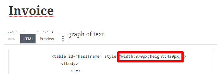
Save your changes by clicking Publish.
Move the calculator 
To move the Custom HTML block to the correct position on the page, drag it using the handle on the left-hand side or use the up/down arrows.
Caching may affect what your visitors see 
If a calculator does not immediately appear on the web, it may be a result of caching. Caching introduces a delay of typically 1-48 hours in the publishing of new or updated content. Read more in the support guide.
Remove the calculator 
To remove a calculator that you previously embedded in page or post:
- Select the Custom HTML block that contains the embed code for the calculator.
- Open the block menu for the block and select Remove Block.
- Save your changes by clicking Publish.
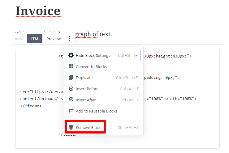 

Embed a spreadsheet with the Classic editor 
Open the Classic editor for the page or post where you want the uploaded calculator to appear.
Place the cursor at the right spot and click Embed SSC Calculator.
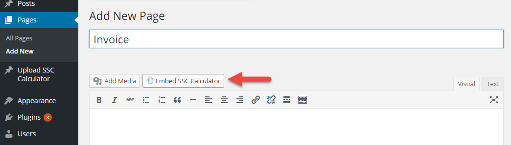
In the list called Calculator Link, scroll to and select the calculator you want to embed.
If necessary, modify the size of the calculator frame in the web page using the fields Iframe Width and Iframe Height. Click Insert Calculator.
If you don’t see the calculator, only a set of HTML tags, click on the Visual tab for a preview of the page.
Change the size of the calculator on the page 
If you cannot see the entire calculator, or if scrollbars appear, or if there’s too much whitespace around the calculator, you may need to adjust the size of the calculator frame. On the Visual tab, locate the resize handle at the lower right-hand corner of the calculator.
Drag the handle to resize the calculator frame.
For better control, switch to the Text tab, adjust the height and width parameters in the <table id=”hasIframe” tag that represents the calculator, switching back and forth to the Visual tab until the calculator looks good. Continue until the calculator looks good. Don’t be afraid of leaving a considerable margin around your calculator.
Save your changes by clicking Publish.
Move the calculator 
To move the calculator somewhere else, e.g. at the bottom of the page, first remove the old embed code using the instructions below, then insert the embed code again where you want the calculator to appear using the instructions above.
Caching may affect what your visitors see 
If a calculator does not immediately appear on the web, it may be a result of caching. Caching introduces a delay of typically 1-48 hours in the publishing of new or updated content. Read more in the support guide.
Remove the calculator 
To remove a calculator that you previously embedded in page or post:
- Switch to the Text mode.
- Remove the entire “hasIframe” table, from the table id=”hasIframe” statement to the /table statement.
- Switch to the Visual mode to verify the result.
- Save your changes by clicking Publish.
Buttons and toolbars 
If you don’t want the calculator to include a toolbar, or if you want to select other buttons for the toolbar, you need to adjust the Workbook settings in SpreadsheetConverter. To remove the toolbar, unselect all buttons in the Workbook > Toolbar section.
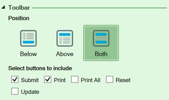
To remove the toolbar, you must also unselect Enable Real-time Sync in Workbook > Web Page Options.

Convert the spreadsheet again and update it in WordPress.
Using the same form or calculator in two or more pages 
If you want to use an uploaded calculator on more than one page, just insert the embed code once for every page where you want it to appear.
Note that by default, each time you embed a form or calculator it will be a unique, independent copy of it. As an example, you may want to add an order form to any page on your website. Any changes you make to the order form on “page A” will not be visible on “page B”, because the two forms are independent. If you want to connect them to show the same order form on two or more pages you may want to read more about the Real-time Sync feature in the “sign-up form” tutorial.
Using forms and calculators in multi-column layouts 
When you create a web form it always appears left-adjusted. If you want to right-adjust it and place text to the left of the form, you need to create a two-column layout for your page. Search the web for wordpress tutorial two columns to get help on how you create a two-column layout first, then move the <iframe> to the correct location in your two-column design.
Support guide 
Still having problems? Try our support guide for the WordPress plugin.
Filling form fields from the link 
Filling form fields from the link 
The link to your web form can contain default values for form input fields, or values set by a script. This help page describes how you use this feature.
You can provide a default or initial value for the fields in an electronic form. Think of it as having a pre-filled link to the form that prepares it with good initial values. Most types of input fields can be pre-filled from the link to the form. The major requirement is that you assign a cell name to each of these cells in the spreadsheet.
All named cells can be set from the surrounding environment, e.g. a script that fetches values from a database. Hidden or locked fields can be used to ensure that the user doesn’t change any sensitive values.
Passing field values in the link or “URL” is technically called a query string. Please note the special technical requirements for query strings and the characters they may contain.
Here are a few examples of links with a query string to set a form field:
- Text field: /form.htm?lang=sv
- Check box: /form.htm?example=TRUE
- Radio button: /form.htm?example=Female
- Ratings: /form.htm?example=4
- Slider: /form.htm?example=42
- Calendar: /form.htm?built_date=20376 (date as Excel serial number) or /form.htm?built_date=10/14/1955 (regional date format)
Known issues 
The form field autosave process normally saves the latest known value for all input fields. The autosaved values from the previous form will override any default values in the link. If you want the values in the link to override the autosaved values, you have to disable Browser Storage on the Workbook tab.
When you share a form with one or more people using Real-time Sync, the contents of the form are preserved during and between sessions. If you provide a value for a form field in the shared link, it will be ignored.
The Workbook tab 
The Workbook tab 
The Workbook tab contains settings that control the conversion of an Excel spreadsheet to a web page.
The Workbook tab of the task pane contains settings for the converted web page. These settings are saved with the spreadsheet.
The contents of the Workbook tab varies slightly between flavors.
This page describes the new layout of the Workbook tab for SpreadsheetConverter version 9 and later. If you are using an older version, please read the help page for version 8.
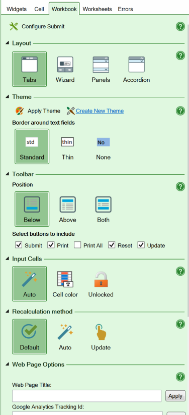
Configure Submit 
If you design an electronic form using an Excel spreadsheet, SpreadsheetConverter can convert it to a smart web form with a free, turnkey solution for the handling of the submitted forms. When a user presses the Submit button in the form, the form’s contents are sent to one of our servers, which converts the form fields into an e-mail and sends it directly to you. The basic functionality is free, giving you immediate access to all the forms submitted by your users.
For a nicer layout, we invite you to a free trial of the Advanced Submit Service. This is a fee-based service that not only makes the e-mail with the form data much easier to read, but also saves all submitted form data on our servers. Whenever you want, you can download this data in one of several convenient file formats.
Click on the Configure Submit link to control how electronic forms are to be handled when submitted.
Read more about how to configure a web form’s Submit options.
Layout 
You select what worksheets in your workbook to show or hide on the Worksheets tab. If you have two or more visible worksheets, you need to specify how the user switches between the sheets.
SpreadsheetConverter has five different ways to handle multi-sheet workbooks:
- Listview shows the sheet names in a list, and you click on a name to view a sheet. (Available in the iPhone/Android flavor only.)
- Tabs generates a tab for each worksheet in the workbook, much like Excel itself does, to let you select what sheet you want to work with. (Available in all flavors except iPhone/Android.)
- Wizard uses Next and Previous buttons in the toolbar to guide the user through a sequential step-by-step data entry process. If you include a bottom toolbar, the Show same height in all pages setting ensures that the bottom toolbar doesn’t move up and down between wizard pages of different length.
- Panels are horizontal headers, each representing a worksheet. When you click on a panel, the corresponding worksheet slides down to appear below it. If you click on the panel again, the worksheet disappears again by sliding in under the panel.
- Accordion layouts are similar to panel layouts but show only one section of the form at a time.
Read more about multi-section forms.


iPhone/Android settings 
Fit page to screen width 
When you create a spreadsheet, you don’t know the exact width of the screen for each user. If you tick the Fit page to screen width checkbox, the web page will always zoom to fill the screen width of any device, both in portrait and landscape orientation. If the checkbox is unticked, a narrow spreadsheet will leave empty screen space to the right, and a wide spreadsheet will require horizontal scrolling.
If you want full control, don’t tick this checkbox, then follow the instructions on how to optimize the Excel column width to fit particular screen widths.
Hide Header and Footer 
The Hide Header and Footer option lets you display just the body part of the spreadsheet in the web page, i.e. without the sheet title, so that it integrates better when you package it with a native app.
Enable Swipe 
The Enable Swipe option is useful when your calculator or form has more than one sheet and it is converted to a web page with the Wizard layout. When Enable Swipe is checked, the user can move between the steps in the wizard by swiping left for Next or right for Previous.
The Mobile settings are only available for the iPhone/Android flavor.
Theme settings 
HTML flavor 
A theme provides layout settings that can be used to tailor the visual appearance of more than one web page. You create a theme with Theme Designer, then import it into your SpreadsheetConverter installation and apply it to one or more spreadsheets before converting them to web pages.
Themes and the Theme Designer are not available for the iPhone/Android flavor.
The Create New Theme link opens the Theme Designer in your default web browser. The Apply Theme link lets you select between the available themes, install a new theme if necessary, then apply it to the current spreadsheet.
Read more about themes and ThemeDesigner.
 

iPhone/Android flavor 
Page Fill Color 
The Page Fill Color is used for the entire background of the converted web page, also in places where there is no corresponding color setting in Excel.
Read more about the Page fill color.
Default Theme 
The Default theme setting allows you to set an overall layout to your web page. There are two settings, Light and Dark.
The Page Fill Color and the Default Theme setting are only available for the iPhone/Android flavor.
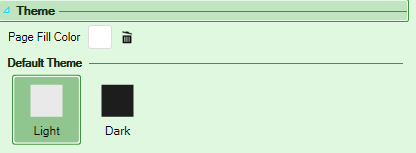 

Borders around text fields 
By default, the text input fields in your web calculators and forms will have a special border that visually indicates that they are open for user input. Output text fields do not have a border unless you have set the corresponding Border property for the cell in Excel.
You can use the Borders around text fields setting to select a thinner border or to remove the border completely. If you remove the border, it will be difficult for the user to see what fields that can be used to enter data, and empty input fields will be invisible.
This option is not available for the iPhone/Android flavor.
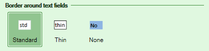

Toolbar position 
SpreadsheetConverter inserts a toolbar in the converted web page. The toolbar contains the action buttons that allow the user to Update a calculator, Submit a form, Print a page or Reset all field contents to their default values.
The Toolbar position setting allows you to place the toolbar Below the spreadsheet, Above the contents of the page, or Both. To completely remove the toolbar, unselect all the action buttons.
The toolbar and this option are not available for the iPhone/Android flavor, which always places the action buttons in the Side Menu.
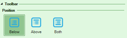
A bottom toolbar normally appears directly below the last content on each page. When using a Wizard layout, the Show same height in all pages setting ensures that the bottom toolbar doesn’t move up and down between wizard pages of different length.
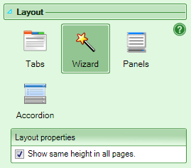
Select buttons to include 
Use the checkboxes under Select buttons to select which of the action buttons you want to include in the toolbar or Side menu.
- When a user has completed entering values into an electronic form, he/she presses the Submit button to send the form for post-processing. The Submit button must be configured to function properly, see Configure Submit above.
- The Print button prints the current worksheet. This option is not available for the iPhone/Android flavor.
- The PrintAll button prints all the sheets in the workbook. This option is not available for the iPhone/Android flavor.
- When a user opens a form that has been used before, the input fields retain the values that were entered the previous time the form was used. The Reset button removes the values from the previous use and restores all field contents to their default values. Most users will consider this rather inconvenient so include this button only if this is a regular need among your users.
- If Automatic recalculation is disabled, the Update button recalculates the cell contents in the spreadsheet. If Automatic recalculation is enabled, this button is redundant.
To completely remove the toolbar, unselect all the action buttons.
You may modify or translate the text for each button using Options > Customize Texts.
In the iPhone/Android flavor, the buttons are located in the Side menu via the “hamburger” button in the top left of the screen. In the other flavors, the buttons are located on the toolbar. Using Action button widgets, action buttons can also be placed almost anywhere on the web page.
Input cells 
When converting a spreadsheet to a web page, SpreadsheetConverter must determine what cells to open for data entry. All other cells are locked in order to protect formulas, captions and constants, and to give the spreadsheet the overall appearance of a web page.
When you design a web form, you may need to manually define certain form fields as input fields to ensure that they will be open for user input in the converted web page. You do this by inserting widgets, using coloring or by unlocking the cells.
Read more about how to open cells for user input.
Recalculation method 
When the user changes anything on the web page, all other cells are normally recalculated automatically, just like with Excel.
For very large spreadsheets, we turn automatic recalculation off to make the web page more responsive – just press an Update button to recalculate the sheet. You can enforce automatic or manual recalculation with the Recalculation Method setting.
Web page options 
This section allows you to assign a few properties that are valid for the entire web page, regardless of what tab or panel the user is on. Always remember to click Apply if you change any of these settings – also if you want to remove a setting by emptying the field.
Web Page title 
You should assign a title for each web page you create. The title appears on the tab for the web page in the web browser.

With many tabs open, you only see the first 15 characters or so of the title. You should put the most distinguishing information in the beginning.
- Don’t use: Order form: Vegetables (If the user also has tabs called Order form: Meat, Order form: Bread and Order form: Fruit, there will be four tabs showing as “Order form:”)
- Do use: Vegetables order form (the other tabs will say Meat order form, Bread order form and Fruit order form.)
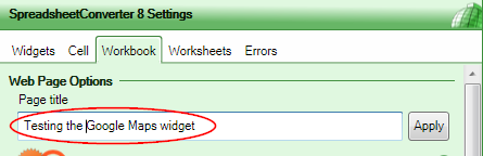
If you don’t specify a page title, the file name is used as the page title.
Google Analytics Tracking ID 
If you use Google Analytics to track your website visitors, please supply your Google Analytics Tracking ID to obtain visitor tracking also for the web pages generated by SpreadsheetConverter. Read more about visitor and conversion tracking.
Google API key 
Google requires you to have an API key to show maps on your website. The API key identifies you as a user of the free map service and allows Google to charge you if you use the service above the free allowance. You can use the same API key for all your Google maps. If you don’t already have one, you can get an API key for free from Google.
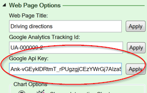
Chart options 
Use the Chart Setting if you want the charts in your web pages to be generated with the old HTML engine. Interactive Charts provide lots of added functionality.
Uncheck the Fixed chart Y-Axis setting to automatically adapt the min and max values of the Y axis in charts to the values.
Enable Real-time Sync 
With Real-time Sync, two or more users can share the same web form or calculator, entering data simultaneously and seeing each other’s changes live on the screen. If you wish to disable Real-time Sync for a calculating web page or web form, untick the Enable Real-time Sync checkbox and convert the spreadsheet again.
Read more about Real-time Sync in the HTML flavor.
Read more about Real-time Sync in the iPhone/Android flavor.

Browser storage 
Web browsers provide a storage feature where websites can save data for later re-use. We use this permanent Browser storage in each of your users’ web browser to save the most recently used field contents for all the web forms the user has visited. If the user opens the same form again, it opens with the most recent values already entered in each field, which can save the user a lot of time. Read more about autosave for forms.
To reset the form fields to their default values, the user can press the Reset button in the toolbar or Side Menu.
If you wish to disable the use of Browser storage for one of your calculators or forms, untick the Enable Browser Storage checkbox and convert the spreadsheet again.
Disabling Browser storage will disable the autosave feature for all form fields, and will also disable the ability to use Offline Forms.
Read more about Browser storage.
 

Hide Lookup range 
If you provide data for lookup operations or dropdown menus in spreadsheet cells, we automatically hide these cell areas on the web page if you tick the Hide lookup range checkbox.

Enable debug mode conversion 
The Enable debug mode conversion setting is mostly used by our developers to obtain more information about a conversion error. It also adds a browser storage toolbar to the converted web page, so that we can get a better look at what’s going on within the browser.
How to change the regional settings in Windows 
How to change the regional settings in Windows 
Most countries in the world use decimal comma (0,1). When you convert spreadsheets for iPhone/Android, you must instead use decimal point (0.1). This help page describes how to change this setting in Windows.
Most people in the world use a point to separate the decimals from the integer portion of a number, but most countries in the world actually use decimal comma.
SpreadsheetConverter normally uses the regional settings in your Windows environment to format numbers correctly for your audience. When converting for mobile devices, however, we need you to use decimal point to ensure correct output. If your system is set for decimal comma, you will get the below error message. Do not press OK at this point.
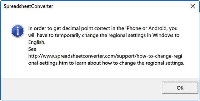
Open the Region control panel 
To open the Region control panel in Windows 8 or later, click on the Windows button in the lower left-hand corner of the screen, then type
Intl.cpl
You can also use Settings > Time & Language > Additional date, time, regional settings > Change date, time, or number formats.
In older Windows systems, open the Run windows by clicking Start > Run, then type the same text and press OK.
If this doesn’t work for you, open the Control panel and locate a control panel for number formats or region.
Change the regional format 
In the Region control panel, select the Formats tab.
Make a note of the current Format: setting.
Change the Format: setting to English (United States).
Click OK to update the regional setting.
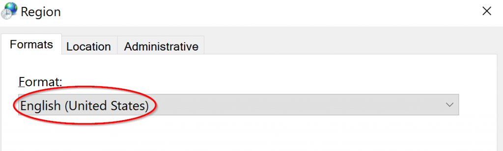
Continue with the conversion 
Return to Excel and the error message that brought you here.
Click OK to continue the conversion with the temporary regional settings or run the conversion again if you’ve already dismissed the prompt to change the regional settings.
Restore your original regional settings 
We recommend that you keep these temporary regional settings until you’ve finished working with the spreadsheet.
Then follow the procedure above again, but this time restore the original Format: setting that is natural for your location.
How to obtain a Google Maps API key 
How to obtain a Google Maps API key 
If you want to show Google Maps on your website, you need an API key from Google. This page shows you how to obtain this key from Google.
When you use the Google Map widget, you are subject to two separate licenses, with two different price models:
- Your use of Google’s map data on your website is tracked and charged for by Google, once for every pageview, with a generous free monthly allowance.
- Your one-time license fee for SpreadsheetConverter includes unlimited use of the Google Maps widget.
To represent your business relationship with Google, they will issue an API key that you need to include in any web page that contains a Google map. The purpose of the API key is to count the number of impressions, i.e. how often your Google maps are viewed on the web. There is a generous free allowance after which Google begins to charge you for additional use of the mapping interface. If you don’t pay, they don’t show any more maps on your behalf until the free usage allowance resets at the end of the month.
This is also true for the maps generated by our Google Map widget. You must enter your own Google API key on the Workbook tab of the task pane for every spreadsheet that contains one or more Google Map widgets. For version 8 or older, you must manually add your API key into the generated code to ensure that the map request is approved by Google.
Obtain a unique Google API key 
After a certain number of free monthly Google map impressions, you will be charged for additional use the same month. Therefore, you must have a Google account and enable this account to use (and if necessary pay for) Google’s map services. You also need a Google API key that you insert in each web page to connect it to the right Google account and its API setup.
If you or your company don’t already have a Google account with a unique Google API key, you must obtain both these things for free from Google. You don’t need a separate API key for use with SpreadsheetConverter. If you already have a working API key, you can use it for all your Google maps.
The API key defines a business relationship between you and Google and looks like this:
Ank-vGEyklDRtmT_rPUgzgjCEzYWrGj7AIzaSyD
It only takes a few minutes to create and it’s something Google requires for their billing.
Login to the right Google account 
Google API keys are part of a Google account. If your Google Maps become popular, you may have to pay for the impressions that exceed your free monthly allowance. You should create your Google API keys within the Google account that uses the credit card you want Google to charge for map views that exceed the free quota.
Before you begin working with your Google API keys, ensure that you are logged in to the appropriate Google account. If you were logged in to your personal account while using YouTube, you may now have to logout and instead login to a corporate Google account before you continue.
The Google API Console 
Now open the Google API Console. This is where you maintain your projects and API keys. It is also here that you enable your Google account for various services like generating dynamic or static maps on your website.
Check if there is already a key available for this Google account. If so, you can use the existing key unless you want to have separate keys for each website or with different restrictions. If you can’t use an existing API key you need to create a new key.
Do not let your credit card expire 
If your credit card expires, your Google maps will stop working on your website. You should set a calendar reminder to update the expiry date every time you get a new card. Otherwise, your maps will look like this:
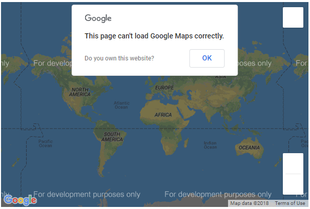
Counting impressions 
Every time you display a map from Google, their servers count this as one use of the API. There is a free allowance after which Google will start to charge you for your use of their software.
Since every impression consumes the free allowance, you may want to use the maps efficiently. As an example, if you want to show a map to help people find your head office, you probably shouldn’t place that map at the bottom of every page in your website, since this would count every single pageview on your website as one use of your free allowance. Instead, place the map only on the About or Contact page. After that, only visits to this specific page will count towards the free limit.
Protecting your API key 
Unfortunately, API keys are valuable. Anyone can copy the API key from your web pages and use them on a different website to get free map views. This use of your API key may eventually have to be paid for by your account. After a while, you may notice that the use of the API is increasing but not the number of visitors to your website, and you may even have to pay for maps that are shown on other people’s websites if they steal your API key and use it so much that it exceeds your free allowance.
To avoid this, you should always restrict your API keys to be valid only for your own domains. Always protect your API keys by using the Accept requests from these HTTP referrers (web sites) option in the Google API console. You should add your domains in two formats: *.example.com/* and example.com/*. With SpreadsheetConverter you should also enable localhost if you want to see Google Maps in the Instant Preview of your web pages directly after conversion.
Here is an actual example of what the list can look like:
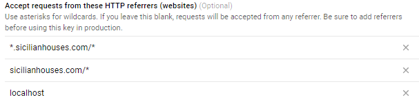
If you will use your web pages on more than one domain, or your website can be accessed using more than one domain name, you must add all these extra domain names to the list as well.
Recovering from a stolen API key 
If one of your API keys is compromised, we recommend that you
- Generate a new key using the Google API Console.
- Set the correct restrictions for the new key.
- Reconvert all your online calculators and forms using the new API key and replace any file on the web that is using the old API key.
- Deactivate the old key using the Google API Console. This will make the old API key useless, also for the people that stole it.
Enable the Google Maps Javascript API 
For detailed instructions, please visit https://developers.google.com/maps/documentation/javascript/get-api-key.
In the Google API Console, you must enable the Google Maps Javascript API for your Google account. With SpreadsheetConverter, this enables you to use Google Map widgets in your forms or calculators.
To verify that your Google account is properly set up to use Google Map widgets with SpreadsheetConverter:
- Open a test spreadsheet with a Google Map widget in it, or create one.
- Insert the Google API key on the Workbook tab of the task pane (see below for instructions).
- Convert the spreadsheet to a web page and open the converted web page in a web browser.
- If the map does not appear correctly in the converted web page, please login to the Google API console and verify that the Google Maps Javascript API is enabled for your Google account, that the API key you have set for the spreadsheet is correct, that you haven’t violated any of the restrictions you have set for this API key and that you haven’t exceeded the usage limits.
Contact our Help Desk if you get stuck.
Enable the Google Static Map API 
For detailed instructions, please visit https://developers.google.com/maps/documentation/static-maps/.
We also recommend that you enable the Google Static Map API for your Google account. This is used when the map is generated as a static image. With SpreadsheetConverter, this is necessary when we deliver static images of maps in the PDF file for a submitted form.
To verify that your Google Static Map API is correctly configured, we recommend that you test inserting a static map on your website. You will need a page where you can insert this map without confusing your website visitors – below we call this the “test” page.
- Edit the test page on your website.
- Copy this entire HTML tag and paste it into the HTML of the test page:
<img src="https://maps.googleapis.com/maps/api/staticmap?center=Brooklyn+Bridge,New+York,NY&zoom=12&size=600x400&key=YOUR_API_KEY" />
- Copy the Google API key you wish to test and paste it directly after &key= in the tag above, replacing the entire placeholder, but retaining the double quote and a blank space before the slash.
- Save the test page and upload it to the web server if necessary.
- Open the test page in a web browser.
- If all is good, your web browser should render the above IMG tag as a static map. If it does not, please login to the Google API console and verify that the Google Static Map API is enabled for your Google account, that the API key you are using on the test web page is correct, that you haven’t violated any of the restrictions you have set for this API key and that you haven’t exceeded the usage limits.
Contact our help desk if you get stuck.
Activate the API key in SpreadsheetConverter 
To use a Google Map in a spreadsheet, open the spreadsheet in Excel. Open the Workbook tab of the task pane and enter your Google Map API key.
If you are using version 1-8 of SpreadsheetConverter, you need to manually add the API key to the converted web page.
Use the Google Map widget 
To insert a Google Map in your spreadsheet, use the Google Map widget.
Help! I need somebody. 
We are always here to help you succeed with SpreadsheetConverter. Please contact our Help Desk if any of your Google Maps don’t appear properly on your website.
Install the WordPress plugin to import spreadsheets 
Install WordPress plugin 
Installation instructions for the WordPress plugin to import spreadsheets.
Install the WordPress plugin to import spreadsheets 
Here are the instructions on how to install the WordPress Plugin to Import Spreadsheets from Microsoft Excel.
Before you attempt to install the WordPress plugin, please read the Requirements section below.
Requirements 
To use the plugin, you need the following:
- A paid or free-trial license for SpreadsheetConverter. The plugin does not import unconverted spreadsheets. An example file is delivered with the plugin.
- Your paid SpreadsheetConverter license must be for the Professional Edition.
- You must use the same major version of the plugin as your SpreadsheetConverter license is for.
- A WordPress server that allows you to install plugins and use iframes. If you use WordPress.com or other hosted environments that limit this, it’s just as easy to use Publish to Cloud instead.
- The plugin requires version 4.5 or later of WordPress. For security reasons, WordPress should always be updated to the latest stable version.
- The plugin supports PHP 5, PHP 7, and PHP 8.
- The ZipArchive extension for PHP must be installed and enabled on your WordPress server.
- You will need the help of a WordPress Administrator or be one yourself to install and maintain the plugin. Unfortunately, we are unable to support you with basic WordPress issues.
Download the plugin file 
Download the plugin directly from the WordPress plugin directory. Remember the location where you save the installation file because you will use it in the next step.
Upload the plugin file to your WordPress server 
Login to the WordPress administration page for your server.
- Click on Plugins in the left-hand menu. If you cannot find this in the menu, contact your WordPress administrator.
- Click on Add New.
- Click on Upload Plugin on the Add Plugin page.
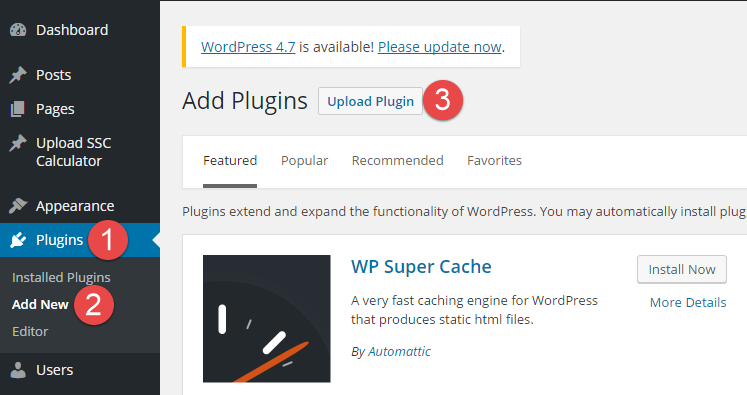
Click on Choose File on the Add Plugin page.
In the File Explorer window,
- Select the plugin zip file that you downloaded in the first step.
- Click Open.
Click on Install Now on the Add Plugin page.
Locate the new plugin in the list of installed plugins and click on Activate Plugin.
The plugin is now installed and active.

You should now see a new menu option Upload SSC Calculator in the left-hand menu. This is where you start when you want to upload a converted calculator to WordPress.
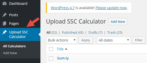
Unfortunately, we are unable to support you in normal day-to-day WordPress activities. If you have problems installing the plugin, begin by contacting your local WordPress Administrator or webmaster. If they find any errors in our plugin, they are welcome to contact our Help Desk.
Manage Uploaded Spreadsheets in the WordPress Plugin 
Manage Uploaded Spreadsheets in the WordPress Plugin 
When you upload spreadsheets to WordPress you may need to update them or remove them. This is the help page for managing uploaded spreadsheets in WordPress.
Updating a calculator to a later version 
Let’s say you have created a calculator and it works fine in your blog. Since then you have edited the spreadsheet in Excel and converted it again. You have also created a new SSC Calculator file. How do you update all the pages on the website that are using the old version, to use the new version instead?
In WordPress, click on Upload SSC Calculator, then All Calculators. Move the mouse cursor over the title of the calculator you want to update, so that its menu links appear. Click on the Edit link. Click Choose Package and select the updated SSC Calculator ZIP file. If you want to use the example file provided with the plugin, it is in the examples > 2-update folder of the plugin ZIP. If you have converted the example yourself, locate the SSC Calculator file that you just created. Press Update. The new version is uploaded and automatically used instead of the old one, in all pages and posts that you have already embedded it.
If you have changed the dimensions of the calculator frame, you may want to drag the resize handle or adjust the height and width parameters of the <iframe> tag in each page (it is visible and editable on the Text tab) until the calculator looks good. (Note: If your WordPress site uses advanced caching, you may have to clear the cache to activate the updated calculator.)
Once the calculator is embedded into a post or page in WordPress, it is automatically replaced when you uplöad an SSC package file with the same name. For example, if you have uploaded a package file named weekly-time-card.zip and embedded it in one or more pages, then you can update it with a new weekly-time-card.zip SSC package file, but not with a package having a different name like invoice.zip.
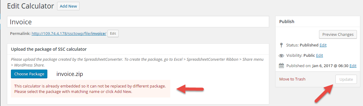
Caching may delay updates to your web pages 
If an update to a calculator does not immediately appear on the web, it may be a result of caching, which is beyond our control. Caching typically introduces a delay of 1-48 hours in the publishing of new or updated web content. Read more in the support guide.
Deleting a calculator you have uploaded but won’t be using 
If you uploaded a calculator to WordPress but won’t be using it, you can easily delete it.
Click on Upload SSC Calculator, then All Calculators. Move the mouse cursor over the title of the calculator you want to delete, so that its menu links appear. Click on the Trash link. If you want to delete two or more calculators, you can also tick the checkbox for all calculators that you want to delete, select Move to Trash in the Bulk Actions menu and press Apply.
Oops, you deleted a calculator by mistake, and now you want it back. This is how you restore it from the Trash:
Click on Upload SSC Calculator, then All Calculators. Just above the first calculator in the list, you will see links for All, Published, Drafts and Trash. Click on the Trash link. Locate the calculator you want to restore in the list and click on its Restore link. If there is no Trash link, or if your calculator is no longer in the Trash, it is because calculators automatically get deleted by WordPress after 30 days in the Trash. If you still have the SSC Calculator file you can just upload the calculator again.
Manually add a Google Maps API key 
Add a Google API key 
You need an “API key” from Google to show Google Maps on your website – including the ones generated by our Google Map widget
Manually add a Google Maps API key 
New Google Maps may not appear as expected on your website. This is because Google requires your API key. Read the instructions on how to solve this.
If you want to show Google Maps on your website, you need an API key from Google. This is also true for the maps generated by our Google Map widget. The purpose of the API key is mainly to count how often your Google maps are viewed on the web. There is a free allowance, after which Google will start to charge you for your use of their mapping software.
When we developed the Google Map widget we felt that the use of it would be minor and that there would be no need for the API key. Until June 2016, Google allowed this, but since then they have hardened their license restrictions. Now we see Google refusing to show maps if the API key is missing. The error message looks like this:

In version 9 of the program, we added the ability to specify the API key on the Workbook tab of the task pane. If you have an older version, you must manually add your API key into the generated code to ensure that the map request is approved by Google. This help page contains the instructions on how to do this.
Obtain a unique Google API key 
You must register as a web user of Google’s services. If you or your company don’t already have a unique Google API key, you can request one for free from Google.
Convert the spreadsheet that contains the widget 
Open a spreadsheet that contains a Google Map widget in Excel. Move to the SpreadsheetConverter ribbon and click Convert to convert the spreadsheet to web format.
Locate the converted web page 
Normally, the converted web page is stored in your Documents > SpreadsheetConverter folder. If you don’t find it, the location may have been changed in the SpreadsheetConverter ribbon > Options > Browsers and Conversion Path Option.
In the folder with the converted web pages, each conversion result is stored twice: 1) uncompressed in a folder and 2) compressed in a ZIP file. We recommend that you delete the ZIP file, then edit the uncompressed version. If you intend to upload the calculator using the WordPress Plugin to Import Spreadsheets from Microsoft Excel you must then compress the updated folder into a new ZIP file before you upload it with the plugin.
Edit the converted web page 
In the folder with the conversion output, you will find a main .htm file that is bigger than the others, with the same name as the spreadsheet, e.g. example.htm. For some flavors, it may instead be called index.htm. Open this file in a text editor.
Search for a section at the end of the page source that looks like this:
<script>document.write("<script type='text/javascript' src='" + (document.location.protocol == 'https:' ? 'https:' : 'http:') + "//map.google.com/maps/api/js' defer></script>");</script>
This is the code we use to generate a Google Map widget on the web page. Now edit this code snippet to look like this:
<script>document.write("<script type='text/javascript' src='" + (document.location.protocol == 'https:' ? 'https:' : 'http:') + "//map.google.com/maps/api/js?key=Ank-vGEyklDRtmT_rPUgzgjCEzYWrGj7AIzaSyD' defer></script>");</script>
The key in bold in the example above is made up, it is just an example and won’t work for you. You must insert your own API key that Google has sent you for the script to work properly.
If you use more than one Google Map widget in the page, all map views will be attributed to the API key you just added. Save the edited file. Compress the entire folder to a ZIP file if this is required when you upload the calculator.
Upload the web page 
There are many ways to upload a converted spreadsheet to a web page and there is no room to document them all here. You may be using FTP against a local website or the WordPress Plugin to Import Spreadsheets from Microsoft Excel. Just follow the same procedure that you used the previous time you uploaded the calculating web page.
Test the web page 
When you have uploaded the web form or calculator and embedded it into your blog or website, open it in your browser and verify that all Google maps appear correctly.
If you still get the error message above, you may be viewing a cached version of the page. Use the View Source option of your web browser to verify that the API key you inserted is indeed present in the HTML source for the web page you are viewing. If it isn’t, clear any caches in your web browser and web server until the API key is really present in the source for the web page.
If the error persists you may need to double-check the file you edited against the instructions above. It is programming code and it must follow the JavaScript syntax requirements.
We are always here to help you succeed with SpreadsheetConverter. Please contact our Help Desk if any of your Google Maps still don’t appear properly on your website.
Repeat for every future conversion 
You need to update this every time you convert the spreadsheet, since every conversion overwrites the previous conversion results.
Saving data in an online spreadsheet 
Saving data in an online spreadsheet 
You can save the data in an online spreadsheet by opening it as a Real-time Sync session. All shared sessions are persistent and the data from the last edit is always there when you open the same session again.
When you use a spreadsheet for calculations, you often want to retain the data from the last time you used the spreadsheet. This is easy using Excel’s Save command, which saves the contents of the spreadsheet to a hard drive or any other type of persistent data storage. If the spreadsheet is saved on a server, many users can access the same spreadsheet and their joint modifications to the spreadsheet are continuously updated on the server.
But how to you keep data in a spreadsheet that has been converted to a web page? Every time your web browser fetches the web page from the web server, it gets the same content – the cell values from when the web page was created. You can change the calculations and get new results, but the next time you open the same web page you start over with the same initial values.
Make your spreadsheet persistent with Real-time Sync 
SpreadsheetConverter provides a simple but genial solution to the problem. When you enable Real-time Sync for a spreadsheet, all its contents become persistent. Every time you open a spreadsheet via Real-time Sync, you get its most recent cell values. This is because Real-time Sync lets two or more people to share a spreadsheet, and these sharing sessions have no limit in time. Even if all users disconnect from a sharing session, Real-time sync still preserves the most recent contents until the next time someone opens the same sharing session again.
It’s time to introduce you to a little trick. The only difference between a standard, unique spreadsheet link and a shared link is the “k” parameter in the link, which is used to provide the unique “key” for the Real-time Sync collaboration session. So if the link to your calculator looks like this:
http://www.example.com/budget/budget.htm
you can create a saved, persistent version just by adding a “k” parameter at the end of the link, like this:
http://www.example.com/budget/budget.htm?k=northwest
In this example, we are using the word “northwest” as the key to, or session name, for our Real-time sync session. The contents of the “budget” spreadsheet are now saved to disk in the online Real-time Sync server. Any change you make to the spreadsheet when opened with this particular key will automatically be retained until you (or someone else) open the same session again, i.e. using the same “k” parameter.
Real-time Sync enables you to collaborate with other people on a spreadsheet, but it also allows you to collaborate with yourself, from one occasion to another. Any online spreadsheet created with SpreadsheetConverter can be made persistent just by adding a session name at the end of the link. There’s no Save button to press, everything is saved while you work.
Learn more 
There is a tutorial for a persistent Sign-up form.
Secure login for Node.js 
Secure login for Node.js 
Secure Login lets you control who can access your Node.js calculator. This is additional layer of protection for your calculator. The first screen anyone sees is the Login page. Your actual calculator page is hidden and cannot be accessed without logging in. Only registered users with a valid password can use your calculator.
Enabling Secure Login 
Activating Secure Login is very simple. You just check the Enable Secure Login Page checkbox in SpreadsheerConverter, Task Pane > Workbook tab > Web Page Options.
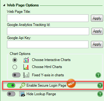
After you have converted the spreadsheet, you should see the Login screen instead of the actual calculator.
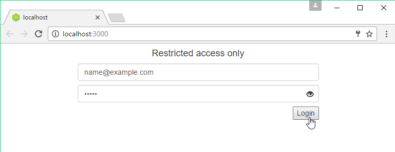
Administrator login 
After the conversion, you will be presented with the initial login credentials for the administrator. There can be only one administrator for each calculator.
The login e-mail for the administrator is the e-mail associated with the registered Node.js license, with the default password admin. You should change this password immediately after you’ve logged into the calculator the first time.
There is no way to recover the administrator’s password, if you have lost it.
Administration interface 
After login, the administrator can add new users, remove existing users and change user passwords.
On the top-right corner of the webpage, there is a user icon with red circle. Clicking on the it, displays the menus: Manage Account and Logout.
Clicking on the Manage Account, opens up a pop-up dialog from where the administrator can add a new user.
To add new users, enter a user name or an e-mail address and a password.
The administrator can remove users that no longer should have access to the calculator. To remove a user, click on the block icon with the red circle.
There is no way to recover a lost password. If a user forgets a password, the administrator must set a new password using the same pop-up dialog.
Registered users can now login to the calculator using their user name and password. It is also possible to log out by clicking on the user icon in the top-right position of the calculator.
The administration tool does not automatically send new or updated login credentials to the respective users. We recommend that the administrator uses a secure method of communicating user names and passwords to users.
Limitations 
- Secure Login is only available for the Node.js flavor.
- Secure Login requires a Professional Edition license.
- A calculator converted with Secure Login cannot be shared with QuickNode Share.
- If you register login credentials registered while using Instant Testing (i.e. with localhost:// in browser address bar), these user names won’t work when you copy the calculator to a public web server.
Support guide for the WordPress plugin 
Support guide for the WordPress plugin 
Here are the instruction on how to handle problems with the WordPress Plugin to Import Spreadsheets from Microsoft Excel.
Since you’re here, it seems you are having problems with our plugin for WordPress. We’re sorry to hear that. Please follow the instructions below to get help from the right person.
Are you just seeing a white screen? 
WordPress administrators jokingly describe this as “the white screen of death”, or just WSOD. It is well documented and you should be able to find good instructions on how to correct this on the web. After you have brought your site back up again, please continue here.
You need a SpreadsheetConverter license key 
The WordPress plugin is only useful for people that use the SpreadsheetConverter add-in for Microsoft Excel, or test it with a trial license. Sometimes we get support requests from people that want to import raw, unconverted spreadsheets into WordPress. Unfortunately, we cannot assist you with that.
Please provide your SpreadsheetConverter Professional edition or trial license key when you report any issues with the plugin.
You need a successfully converted spreadsheet 
Before you report any issues with the plugin, you need to have an Excel spreadsheet that has been successfully converted to a web page with SpreadsheetConverter.
You must have the plugin installed and functional 
You must install the plugin according to the instructions in the Installation guide.
Unfortunately, we are unable to support you in normal day-to-day WordPress activities. If you have problems installing the plugin, begin by contacting your local WordPress Administrator or webmaster.
You should see “Upload SSC Calculator” in the left-hand menu 
If you cannot use the plugin, you may have had installation problems that you didn’t notice. Go back and try the installation again.
Check if you have one of the known issues 
There are a few issues that we know may cause problems. Please check if your problem is one of the below:
- The plugin requires that the ZipArchive extension for PHP is installed and enabled. Consult your webmaster or hosting provider to install or activate ZipArchive.
- When using the Classic editor in Google Chrome, an embedded calculator may disappear from the page/post that is being edited. If you need to use the Classic editor, use another web browser like Edge or Firefox. Read more in the Upgrade Notice in the plugin’s ZIP file.
Verify that the problem is caused by the plugin 
It’s easy to deactivate all of your plugins using the bulk action option at the top of the main plugins page i.e. www.example.com/wp-admin/plugins.php. If you still have the problem, at least you now know it is not caused by one of your plugins.
Now enable only the Import Spreadsheets from Microsoft Excel plugin and test again. If the problem has returned, it is probably caused by our plugin. Please contact our help desk.
Caching may delay the publishing of new content 
Most WordPress websites are cached to shorten response times. This means that the webpages are stored as pre-rendered, static HTML files that are rapidly accessible for web browsers, without invoking the cumbersome WordPress process to reformat the page for every request. Your website may even be using a Content Delivery Network to host your web pages in multiple locations worldwide. bringing your cached content closer to its global audience.
Each level of caching delays the publishing of new or updated content. The typical publishing delay caused by caching is 1-48 hours.
When you upload a new version of a calculator, it may not appear immediately in the preview pane of the plugin or in your web pages. This is usually a result of caching, which is beyond our control.
When you test static content like uploaded calculators, you can try adding a fake “version” parameter to the link to the calculator:
https://example.com/calculator.html?version=1
When you update the calculator, just remember to change also the version number in the links to it, which should force the cache to fetch the updated content. Note: you only need the version parameter during testing, to verify that the update went through correctly. In your production environment, the updated version will be loaded automatically when the cached copies of the previous version expire.
If this doesn’t work for you, you should contact the person responsible for your caching setup and request that each cache is purged, so that your most recent WordPress updates are made available instead. The main effects of caching appear during the first hour so any additional delay usually has very little impact on response times.
Check if you have a conflict between plugins 
If the problem does not reappear when you enable just the Import Spreadsheets plugin, enable your other plugins one by one until the problem reappears. There may be a conflict between another plugin and the Import Spreadsheets plugin. Please contact our help desk and report the plugin conflict.
Enable and examine your Debug Log 
Your WordPress debug log may contain more information that can help solve the problem. If you haven’t already enabled it, open your wp-config.php file, and ensure you have the following setting:
define(‘WP_DEBUG’, true);
The debug log is in the WordPress content folder. This is usually called wp-content. Open the log file debug.log, go to the bottom and look for log entries that coincide with your recent site interactions.
Check if you have other common WordPress problems 
There are many common problems in WordPress. Please check if your problem is one of the below. To learn more about each problem, please search the web. All these issues are well documented
- Many problems with WordPress, in particular http 500 internal server errors, can be caused by a corrupt .htaccess file. Delete the current file via FTP and upload the last safe version of it from your backups.
- You may be reaching your CPU or memory limits, or the maximum execution time. Consult your webmaster or hosting provider to verify your current settings.
- The core WordPress files may be corrupted. Re-upload all core WordPress files to ensure they are correct.
Contact our help desk 
If none of the above applies to you, please contact our help desk and report the problem you are having. If possible, please include all the details about your server environment including the operating system and version, the PHP version, the WordPress version and the plugin version.
Advanced settings in version 8 
Help: Advanced settings 
This is the Online Help page for the advanced settings in SpreadsheetConverter
Advanced settings in version 8 
The Options menu allows you to use SpreadsheetConverter with other languages than English. It also lets you adjust the advanced conversion settings.
The Preferences section of the ribbon contains various options and settings.
Customize Texts 
You can translate SpreadsheetConverter to other languages or change the texts it uses with the Customize Texts setting. Select the group in the left-hand pane and edit the texts in the group in the right-hand pane. The new texts will be used for all subsequent conversions, but will not affect already converted web pages.
Note: in version 9, these settings were moved to the User Settings page.
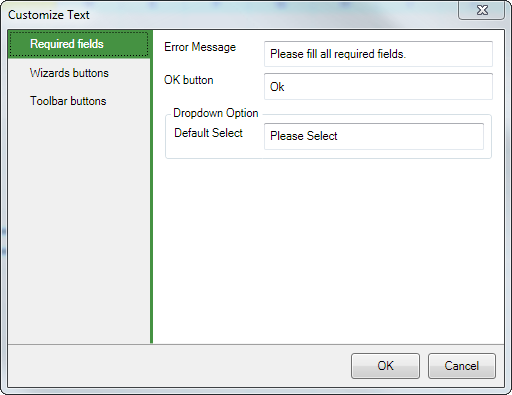
Advanced settings 
The Advanced Settings control the internal operation of the converter. Note: in version 9, most of these settings were moved to the Workbook tab of the task pane.
- If you provide data for lookup operations or dropdown menus in spreadsheet cells, we automatically hide these cell areas on the web page if you tick the Hide lookup range checkbox.
- Uncheck the Fixed chart Y-Axis setting to automatically adapt the min and max values of the Y axis in charts to the values.
- The Combine JavaScript and CSS files setting makes the converted web page smaller and faster to download.
- If you use Google Analytics to track your website visitors, please supply your Google Analytics Tracking ID to obtain visitor tracking also for the web pages generated by SpreadsheetConverter. Read more about visitor and conversion tracking.
- When the user changes anything on the web page, all other cells are normally recalculated automatically, just like with Excel. For very large spreadsheets, we turn automatic recalculation off to make the web page more responsive – just press an Update button to recalculate the sheet. You can enforce automatic or manual recalculation with the Recalculation Method setting.
- Use the Chart Setting if you explicitly require the charts in your web pages to be generated with the old Adobe Flash plug-in. Many mobile devices don’t support Flash, which is why we switched to generating the charts with HTML5.
- If you’ve changed things and want to return to the factory defaults, just press the Reset User Setting button.
- The Enable debug mode conversion setting is mostly used by our developers to obtain more information about a conversion error. It also adds a browser storage toolbar to the converted web page, so that we can get a better look at what’s going on inside the browser.
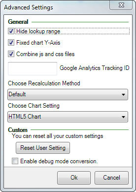
Help: The File Attachments widget 
The File Attachments widget lets your users include up to ten files with any form they submit.
This is the help page for the File Attachments widget.
To learn more about how you can create web forms with SpreadsheetConverter or have them sent to your e-mail inbox, please read the introduction to forms handling.
The File Attachments widget 
Introduction 
The File Attachments widget enables your visitors to include documents, charts, images, videos or any other kinds of files with their form submission. Job applicants can include their CV, and expense reports can include scanned copies of receipts. Users may even use their phone to take a picture and include this with the form.
Any form that you create with SpreadsheetConverter can have file attachments. In the spreadsheet, you insert the widget in a cell that should be wide enough to function well with drag-and-drop.

As the user selects files to include with the form, they are automatically uploaded. The widget shows a list of the files and allows already uploaded files to be removed.

When the form is submitted, the file attachments normally appear as attachments to the e-mail with the form contents.
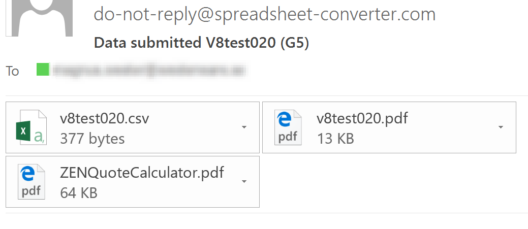
In the Advanced server, the file attachments appear as links from the submitted form.
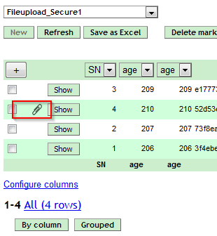
Inserting the File Attachments widget 
To use file attachments in a web form, you must insert a File Attachments widget in a cell in the spreadsheet that you use to design the form.
The File Attachments widget enables users to drag-and-drop files to the form, or click on the text link to select files from a list.
We recommend that you make the widget’s cell big enough to be comfortably used when dragging and dropping files from other windows. You can expand the cell’s area by widening the row and column, by merging adjacent cells, or both.
When you move the mouse pointer over the cell, the mouse pointer changes into hand sign, the text is underlined and a dashed line appears around the cell to show that the widget also lets you drag-and-drop files on it.

The widget lets visitors add up to ten files to any form. In most environments, you can add more than one file at a time.
- In desktop systems you click to select the first item in a contiguous list of files, then hold down the Shift key and click on the last item to be included in the selection. You can also click on the first file, then hold down the Ctrl or Command key while you click to select discontiguous additional files, one at a time.
- In the iOS image browser in iPhone or iPad, you touch images to select or deselect them before you press OK to add all the selected files to the widget.
- In Android you can add both images and other files from the file system.
To save time, the files automatically start to upload as you add them to the widget. There is a progress bar for each file to show how much of it has been uploaded. Until the upload has finished, the file name is faded.

To abort an upload, click on the red delete icon to the right of the file name.
Once the upload is finished, the progress bar goes away and the file name is not faded anymore. To remove an uploaded file, click on its red delete icon.
When the user saves the form, only the form contents remain to be sent. All the attached files have already been sent to the server and are linked to the form.
Formatting the widget 
Introduction 
When you insert the widget into the cell, a default text “Drop your file here or click to browse” appears in the cell and the widget’s properties panel opens in the task pane.
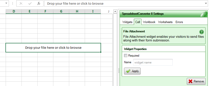
You can change the prompt or translate it to another language simply by editing the text in the cell.
If you select the Required check-box, all users of the form must attach at least one file before they can submit the form.
The text and cell formatting for the File Attachments widget is set using Format Cells in Excel. If you want to have the prompt aligned differently, e.g. centered both horizontally and vertically, adjust the Format Cells settings accordingly.
The cell will appear almost the same in the web page as in the spreadsheet:
but with a paperclip icon to the left of the text.
Using Theme Designer 
A few of the graphical elements used by the File Attachments widget are not managed by Excel, but you still have control over them using the Theme Designer.
In Theme Designer, you can select a Brand color for your theme, and this is used for the paperclip icon, the file icons and the dashed line that appears around the field when you hold the mouse pointer over it. To apply the theme, download it from the Theme Designer and apply it with the Apply Theme setting on the Workbook tab in the SpreadsheetConverter Task Pane.
There are few parts which currently cannot change color. For example, the delete button is always red and the progress bar is always green.
Limitations 
- The File Attachments widget is only supported with the Professional edition of SpreadsheetConverter. Upgrade to the Professional edition to use this powerful widget, lots of new chart types, more Excel functions and many other advanced features.
- The File Attachments widget requires the Advanced Submit Service. Upgrade to the Advanced Submit Service to use this powerful widget and Secure Delivery. The e-mail looks exactly like the form did when the user entered data into it, including graphics and charts. Save incoming web forms in a hosted database. Filter, sort and download saved forms whenever you like.
- You cannot add files to the File Attachments widget while you’re offline. File attachments are supported by Offline Forms but only if you attach the files while you’re online.
- You can insert File Attachments widgets in up to ten places in a spreadsheet.
- Your users can attach up to ten files for each File Attachments widget in the web form.
- Each file that a user attaches to a web form can be up to four megabytes in size.
- After files have been attached to a form, the form must be submitted within seven days. Uploaded files that don’t belong to a submitted form are removed after seven days. Uploaded files that belong to a submitted form are retained forever.
Limitations in the e-mail infrastructure 
When we attempt to deliver the form with its attachments to the designated recipients, the e-mail infrastructure may refuse to deliver it. This is because some e-mail servers limit the size of attachments and/or the entire e-mail. If the user of the web form has attached many large files to the form, the entire package may exceed the limitations imposed by the e-mail infrastructure.
The e-mail infrastructure is beyond our control and there is simply no way for us to guarantee that you will get all the e-mails we send you. The risk of losing e-mails increases when you use File Attachments.
If you use a form that permits File Attachments, we recommend that you use our Secure Delivery feature to have the e-mail contain just a link to the form instead of the form’s full contents with attachments. Clicking on the link in the Secure Delivery e-mail takes you to the server where you can login to access the form and its attachments securely.
The Excel ribbon menu 
Help: Excel ribbon menu 
This is the Online Help page for the SpreadsheetConverter ribbon menu in Excel
The Excel ribbon menu 
The Excel menu contains a separate ribbon for SpreadsheetConverter. This is the online help page for that ribbon menu.
After you have installed SpreadsheetConverter, a new ribbon or menu appears in Excel.
This page describes the ribbon menu for SpreadsheetConverter version 9. If you are using a later version, please read the updated help page for version 10 and later.
If there is no SpreadsheetConverter entry in your Excel menu, please follow these troubleshooting instructions.
Conversion section 
Use the Conversion section of the ribbon to select what flavor to use for the conversion, i.e. what format to use for the converted web page.
After you’ve selected the right flavor, press Convert to convert the current spreadsheet to a live, calculating web page. There is a tutorial to guide you through your first conversion.
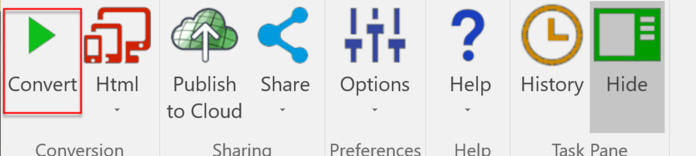
We offer you a free 7-day test of SpreadsheetConverter with access to all flavors in a limited, “demo” mode. You can also request a free 30-day trial license.
After the trial period has ended, unlicensed flavors will no longer appear in the list. If you need a particular flavor, ensure you have a license key for it and that you have activated this license key under Product Activation in the Help menu. There is an online Help page for license registration.
Note that changing the flavor may affect other settings, e.g. for layout and formatting, and some widgets are only relevant in certain flavors.
Sharing section 
The Sharing section of the ribbon helps you publish the converted web page on various external servers. You must convert your spreadsheet before you can share the converted web page.
The choices available depend on what flavor you use, so you may not see all the below in your particular setup.
Publish to Cloud 
Publish to Cloud is a simple and very convenient way to publish your calculator on one of our web servers.
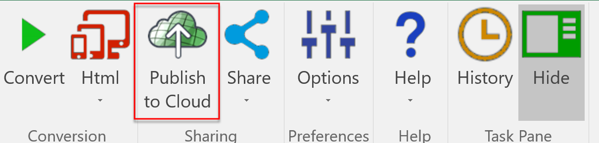
The Share menu 
The Share menu contains different uploading tools depending on your flavor.
WordPress Share 
Some flavors include WordPress Share which makes it much easier to upload your calculator to WordPress using a plugin.
QuickNode Share 
If you have a license for the Node.js flavor, the Quicknode Share service will upload your web page for testing on one of our Node.js servers. There is no charge but the web page is automatically deleted after seven days.
Dropbox Share (discontinued) 
Older versions had a Dropbox Share feature to upload the converted web page for testing in a Dropbox account. Unfortunately, Dropbox has discontinued the ability to host web content.
Preferences section 
The Preferences section of the ribbon contains various options and settings.
Browsers and Conversion Path Option 
- Click on the button to the right under Choose folder to store webpage and navigate to where you want SpreadsheetConverter to store the web pages it creates. All converted web pages are stored in this folder, even if the source spreadsheets are in different folders. Each converted calculator or form will be enclosed in its own subfolder.
-
- Select what browsers you wish to use with Instant Testing to verify the result of each conversion in – click once to activate a browser, click once again to deactivate. Your converted web pages will open in all selected browsers directly after conversion.
User settings 
The User Settings are available in version 9 and later. Read more on the help page for the user settings.
ASP.NET Settings 
For the ASP.NET flavor, the converted web page must be copied to the location on the server where the Site is located. If this drive is available when you do the conversions, you can select the right location directly in the Choose folder to store webpage setting above.
The Choose url setting should be set to match the address of the Site in IIS. For example, if the Site in IIS is configured to listen to port 8080 and the Site name is ‘ssc’ then the correct URL is http://localhost:8080/ssc.
Use the Choose File Format setting to specify whether you want the converted web page to be generated for ASP.Net or Classic ASP.
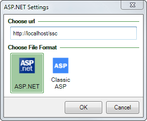
Customize Texts, Advanced settings 
These menu choices can be found in version 8 and earlier versions. Read more on the help page for the advanced settings in version 8.
Purchase Full License Keys 
Follow this link to the license web shop where you can buy the licenses you need to activate the full power of the product. Learn more in the license tutorial.
Check for New Version 
Before you report any technical problems to us, please ensure that you are using the latest version of SpreadsheetConverter. Otherwise you may be reporting a problem that has already been fixed. The Check for New Version menu selection will automatically verify the version you have installed, and help you apply any updates.
Show Announcements in Task Pane 
The announcements in the Notification Center help us communicate new features to you without the use of e-mails, blogs or newsletters. Read more about the Notification Center and how to use it.
Help section 
Use the Help menu to research any problems you might have.
- Take the Tour, a collection of images and descriptive text that helps you get started.
- We deliver a set of Examples with the product. Use this link to browse the examples folder and open some of the examples in Excel. Press Convert to see what each example looks like as a web page!
- The Online Help link takes you directly to the help section of this website.
- Use Contact Support to open a new support ticket at our Help desk.
- Use the Product Activation page to register license keys. For upgrades, you may need to register old license keys as well.
- Follow the Visit our website link to, well, visit our website.
- Open the About box with the currently installed version number which is useful when you contact the Help desk.
Task Pane section 
The task pane is a resizeable work area to the right of the spreadsheet you’re working with.
History menu 
When the History List is shown in the task pane, it contains your most recently converted spreadsheets.
The most recently converted web page is at the top of the History list. To the left of the file name is an icon that tells you what flavor was used to create it, i.e. its output format. Using the buttons below the file name, you can open the web page in any of your web browsers, or in the Windows Explorer. You can also get a QR code for Instant Testing, and use the camera to scan the code to test a calculator in your smartphone.
There is a video tutorial for the History List in version 8.
Show/Hide 
The SpreadsheetConverter task pane is pretty wide and can occupy a significant portion of the screen in Excel. The Task Pane section of the SpreadsheetConverter menu allows you to Show the task pane when you need it and Hide it when it’s no longer needed.
The Workbook tab in version 8 
The Workbook tab in version 8 
The Workbook tab contains settings that control the conversion of an Excel spreadsheet to a web page.
The Workbook tab contains settings for the converted web page. These settings are saved with the spreadsheet.
The contents of the Workbook tab varies slightly between flavors.
This page describes the Workbook tab for SpreadsheetConverter version 8. If you are using a later version, please read the updated help page for version 9 and later.
Page title 
When someone opens the converted web page in a web browsers, the Page title is shown in the Name bar for the browser tab or window. If you don’t specify a page title, the file name is used as the page title.
Enable Real-time Sync 
With Real-time Sync, two or more users can share the same web form or calculator, entering data simultaneously and seeing each other’s changes live on the screen. If you wish to disable Real-time Sync for a calculating web page or web form, untick the Enable Real-time Sync checkbox and convert the spreadsheet again.
This option is not available for the iPhone/Android flavor.
Read more about Real-time Sync in the HTML flavor.
 

Browser storage 
Web browsers provide a storage feature where websites can save data for later re-use. We use this permanent Browser storage in each of your users’ web browser to save the most recently used field contents for all the web forms the user has visited. If the user opens the same form again, it opens with the most recent values already entered in each field, which can save the user a lot of time. Read more about autosave for forms.
To reset the form fields to their default values, the user can press the Reset button in the toolbar or Side Menu, see below.
If you wish to disable the use of Browser storage for one of your calculators or forms, untick the Enable Browser Storage checkbox and convert the spreadsheet again.
Disabling Browser storage will disable the autosave feature for all form fields, and will also disable the ability to use Offline Forms.
Read more about Browser storage.
 

Mobile settings 
Fit page to screen width 
When you create a spreadsheet, you don’t know the exact width of the screen for each user. If you tick the Fit page to screen width checkbox, the web page will always zoom to fill the screen width of any device, both in portrait and landscape orientation. If the checkbox is unticked, a narrow spreadsheet will leave empty screen space to the right, and a wide spreadsheet will require horizontal scrolling.
If you want full control, don’t tick this checkbox, then follow the instructions on how to optimize the Excel column width to fit particular screen widths.
Enable Swipe 
The Enable Swipe option is useful when your calculator or form has more than one sheet and it is converted to a web page with the Wizard layout. When Enable Swipe is checked, the user can move between the steps in the wizard by swiping left for Next or right for Previous.
Hide Header and Footer 
The Hide Header and Footer option lets you display just the body part of the spreadsheet in the web page, i.e. without the sheet title, so that it integrates better when you package it with a native app.
The Mobile settings are only available for the iPhone/Android flavor.
Theme settings 
HTML flavor 
A theme provides layout settings that can be used to tailor the visual appearance of more than one web page. You create a theme with Theme Designer, then import it into your SpreadsheetConverter installation and apply it to one or more spreadsheets before converting them to web pages.
Themes and the Theme Designer are not available for the iPhone/Android flavor.
The Create New Theme link opens the Theme Designer in your default web browser. The Apply Theme link lets you select between the available themes, install a new theme if necessary, then apply it to the current spreadsheet.
Read more about themes and ThemeDesigner.

iPhone/Android flavor 
Page Fill Color 
The Page Fill Color is used for the entire background of the converted web page, also in places where there is no corresponding color setting in Excel.
Read more about the Page fill color.
Default Theme 
The Default theme setting allows you to set an overall layout to your web page. There are two settings, Light and Dark.
The Page Fill Color and the Default Theme setting are only available for the iPhone/Android flavor.

Borders around text fields 
By default, the text input fields in your web calculators and forms will have a special border that visually indicates that they are open for user input. Output text fields do not have a border unless you have set the corresponding Border property for the cell in Excel.
You can use the Borders around text fields setting to select a thinner border or to remove the border completely. If you remove the border, it will be difficult for the user to see what fields that can be used to enter data, and empty input fields will be invisible.
This option is not available for the iPhone/Android flavor.
Layout 
You select what worksheets in your workbook to show or hide on the Worksheets tab. If you have two or more visible worksheets, you need to specify how the user switches between the sheets.
SpreadsheetConverter has five different ways to handle multi-sheet workbooks:
- Listview shows the sheet names in a list, and you click on a name to view a sheet. (Available in the iPhone/Android flavor only.)
- Tabs generates a tab for each worksheet in the workbook, much like Excel itself does, to let you select what sheet you want to work with. (Available in all flavors except iPhone/Android.)
- Wizard uses Next and Previous buttons in the toolbar to guide the user through a sequential step-by-step data entry process. If you include a bottom toolbar, the Show same height in all pages setting ensures that the bottom toolbar doesn’t move up and down between wizard pages of different length.
- Panels are horizontal headers, each representing a worksheet. When you click on a panel, the corresponding worksheet slides down to appear below it. If you click on the panel again, the worksheet disappears again by sliding in under the panel.
- Accordion layouts are similar to panel layouts but show only one section of the form at a time.
Read more about multi-section forms.
Input cells 
When converting a spreadsheet to a web page, SpreadsheetConverter must determine what cells to open for data entry. All other cells are locked in order to protect formulas, captions and constants, and to give the spreadsheet the overall appearance of a web page.
When you design a web form, you may need to manually define certain form fields as input fields to ensure that they will be open for user input in the converted web page. You do this by inserting widgets, using coloring or by unlocking the cells.
Read more about how to open cells for user input.
Toolbar position 
SpreadsheetConverter inserts a toolbar in the converted web page. The toolbar contains the action buttons that allow the user to Update a calculator, Submit a form, Print a page or Reset all field contents to their default values.
The Toolbar position setting allows you to place the toolbar Below the spreadsheet, Above the contents of the page, or Both.
The toolbar and this option are not available for the iPhone/Android flavor, which always places the action buttons in the Side Menu.
A bottom toolbar normally appears directly below the last content on each page. When using a Wizard layout, the Show same height in all pages setting ensures that the bottom toolbar doesn’t move up and down between wizard pages of different length.
Select buttons to include 
Use the checkboxes under Select buttons to select which of the action buttons you want to include in the toolbar or Side menu. You may modify or translate the text for each button using Options > Customize Texts.
- When a user has completed entering values into an electronic form, he/she presses the Submit button to send the form for post-processing. The Submit button must be configured to function properly, see Configure Submit below.
- The Print button prints the current worksheet. This option is not available for the iPhone/Android flavor.
- The PrintAll button prints all the sheets in the workbook. This option is not available for the iPhone/Android flavor.
- When a user opens a form that has been used before, the input fields retain the values that were entered the previous time the form was used. The Reset button removes the values from the previous use and restores all field contents to their default values.
- If Automatic recalculation is disabled, the Update button recalculates the cell contents in the spreadsheet. If Automatic recalculation is enabled, this button is redundant.
In the iPhone/Android flavor, the buttons are located in the Side menu via the “hamburger” button in the top left of the screen. In the other flavors, the buttons are located on the toolbar. Using Action button widgets, action buttons can also be placed almost anywhere on the web page.
Configure Submit 
If you design an electronic form using an Excel spreadsheet, SpreadsheetConverter can convert it to a smart web form with a free, turnkey solution for the handling of the submitted forms. When a user presses the Submit button in the form, the form’s contents are sent to one of our servers, which converts the form fields into an e-mail and sends it directly to you. The basic functionality is free, giving you immediate access to all the forms submitted by your users.
For a nicer layout, we invite you to a free trial of the Advanced Submit Service. This is a fee-based service that not only makes the e-mail with the form data much easier to read, but also saves all submitted form data on our servers. Whenever you want, you can download this data in one of several convenient file formats.
Click on the Configure Submit link to control how electronic forms are to be handled when submitted.
Read more about how to configure a web form’s Submit options.
Upload a spreadsheet to WordPress 
Upload a spreadsheet to WordPress 
These instructions will show you how to convert a spreadsheet to a live web calculator and upload it as an SSC Calculator file to WordPress.
The WordPress Plugin to Import Spreadsheets from Microsoft Excel makes it easy to upload converted calculators and web forms to WordPress and embed spreadsheets in any post or page.
When you upload a spreadsheet to WordPress, you first convert it to web format with SpreadsheetConverter. Then you upload the result of the conversion to WordPress in the form of an SSC Calculator file. The SSC Calculator file contains everything that WordPress needs to run the calculator.
WordPress prohibits most special characters in file names. Please note the rules for input filenames before you continue.
Follow these instructions only when you upload a new calculator for the first time. If you later want to update an existing calculator that you have already uploaded at least once to WordPress, read the separate instructions for this.
Create the SSC Calculator file 
With the plugin, you get two example files, one that you can use for this initial upload and one to test how to update an existing calculator. If you want to create the example files yourself, and have downloaded and installed the Excel add-in, please do the following:
Activate a paid Professional edition license for SpreadsheetConverter, or request and activate a free-trial license key.
Open the “Weekly Time Card” example spreadsheet and convert it to a web page according to the instructions on the Download page. Leave the example file open in Excel and allow the conversion to finish.
In Excel, select the SpreadsheetConverter ribbon and click on the WordPress plugin button in the Publish section. Note: Click in the middle of the button to avoid the little downward arrow to the right that just opens a list of integration tutorials.
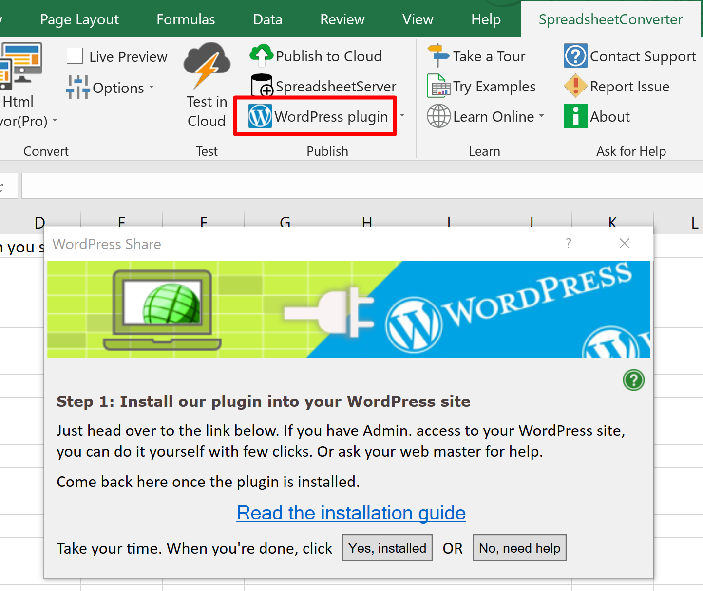
This will start a short wizard that on the first run ensures that you have installed the WordPress Plugin to Import Spreadsheets from Microsoft Excel. It then creates the SSC Calculator file for you.
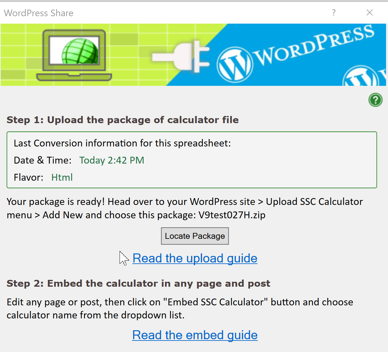
To keep track of the SSC Calculator file, you may click on the Locate Package button to open its surrounding folder in the File Explorer. By default, this will open Documents > SpreadsheetConverter.
Upload a converted spreadsheet 
(Follow the Add New instructions below only for the first, initial upload of each calculator. After that, follow the instructions on how to update an existing calculator instead.)
Now leave Excel and move over to your web browser and log in to WordPress.
After a successful installation of the plugin, there will be an Upload SSC Calculator link in your WordPress menu. If you don’t see this link, please verify that you have installed the plugin correctly.
Click on Upload SSC Calculator, then click Add New to upload a new calculator.
- Enter a unique, descriptive name for this particular calculator in the Enter Calculator Name field. For the example file, you can use Weekly Time Card.
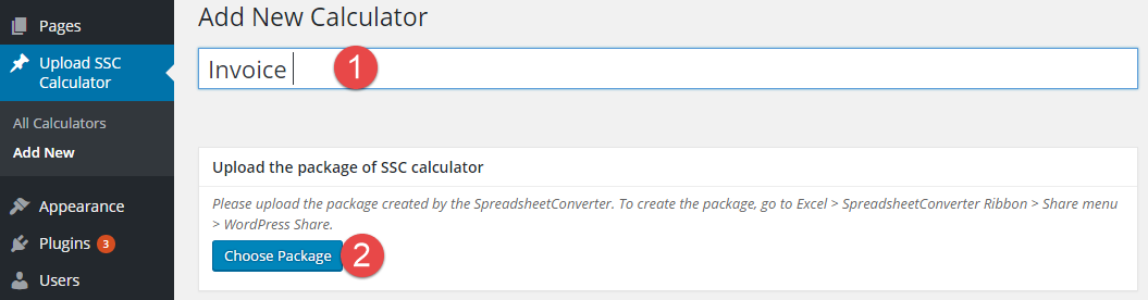
- Click on Choose Package and select the SSC Calculator file. If you want to use the example file provided with the plugin, it is in the examples > 1-upload folder of the plugin ZIP. If you have converted the example yourself, locate the SSC Calculator file that you just created. By default, it is located in Documents > SpreadsheetConverter. If your calculator is called weekly-time-card.xlsx, there will be a folder called weekly-time-card with your converted calculator. You cannot upload this uncompressed folder, only the specially prepared and compressed SSC Calculator file which is in ZIP format. Scroll down past the folder to the weekly-time-card.zip file, select it and press Open. If you cannot find the SSC Calculator .ZIP file for the web page, ensure that you have created it using the instructions under Create the SSC Calculator file above and that you are looking in the same folder that the Locate Package button opened for you above.
- Press the Publish button and the SSC Calculator file will be uploaded to WordPress. It will not be visible in any post or page until you embed it.
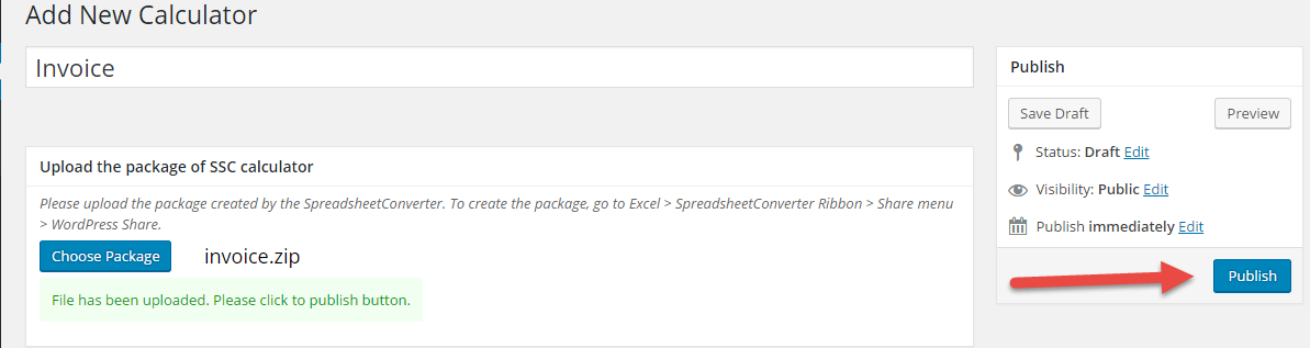
Next step 
Now you’re ready to embed the calculator in your website.
The fine print 
The WordPress plugin only uploads calculators from the same version of SpreadsheetConverter. For example, if your calculator was converted with version 10 of SpreadsheetConverter, you must use version 10 of the WordPress plugin to upload it.
The SSC Calculator file gets its name from the original spreadsheet and cannot be renamed. To change the name of the SSC Calculator file, create a copy of the original spreadsheet with the name you prefer before you convert it again.
Support guide 
Still having problems? Try our support guide for the WordPress plugin.
The WordPress plugin to import spreadsheets 
The WordPress plugin to import spreadsheets 
Here are the instructions on how to use the WordPress Plugin to Import Spreadsheets from Microsoft Excel.
We offer a free WordPress plugin that allows you to import live, calculating spreadsheets from Microsoft Excel to your blog or website in WordPress. To use the plugin, you need a web page created with the Professional Edition edition of SpreadsheetConverter. An example file is delivered with the plugin.
Note: You can also publish spreadsheets from Microsoft Excel in WordPress using our Publish to Cloud service. The main difference is that the calculator then resides on a cloud server and not on the same web server as your WordPress site. In most cases, this works just as well.
Using the plugin 
Insert a live spreadsheet in your blog with just a few clicks 
Any Excel spreadsheet can be published on the web. It’s probably easiest to start with the example file provided with the plugin. If you’re already familiar with SpreadsheetConverter, you can also convert the example file to an SSC Calculator file yourself:
- If necessary, download and install the Excel add-in using the instructions on the download page. In Excel, select the SpreadsheetConverter ribbon and verify that there is a WordPress plugin button in the Publish section.
- Open the spreadsheet in Excel and click Convert> on the SpreadsheetConverter toolbar to convert the spreadsheet to a web page.
- Click WordPress plugin on the SpreadsheetConverter toolbar to create an SSC Calculator file with everything you will need in WordPress.
Once you have the SSC Calculator file, you move over to WordPress:
- Use the WordPress plugin to upload the SSC Calculator file to WordPress.
- Embed the calculator or form into one or more of your posts or pages in WordPress.
- Click Publish in WordPress and your calculator goes live, online on the web!
Install the plugin 
Before you publish your first calculator, you must install the plugin in WordPress with help from the instructions in our Installation Guide.
Manage the uploaded calculators 
If you want to move a calculator within the page, or to another page, there’s much to learn in the Manage Uploaded Spreadsheets section, which also tells you how to completely remove a calculator from WordPress.
Support guide 
Still having problems? Try our support guide for the WordPress plugin.
Help: Use Offline Forms 
Old offline forms may cease to work 
In 2015 we introduced an offline forms feature built on a web standard called AppCache that is now being deprecated. We want you to be aware that depending on your web browser, AppCache-based offline forms may cease to work at some point in the future.
Our developers are investigating a new implementation. If and when such an implementation appears, you will need to upgrade to the then current version of SpreadsheetConverter and use it to re-convert your offline forms to use the new functionality.
Please contact our help desk if you have any questions regarding the future support for offline forms in SpreadsheetConverter.
With offline forms, users can submit forms even when they are not connected to the Internet. The forms are saved inside the web browser. When users get back online, they just press a button to submit all their queued forms. Follow these steps to save multiple forms in the web browser and later have them all submitted at once.
Note that the offline submit doesn’t work when you’re connected to the Internet. We never save any forms as long as they can be submitted directly.
Before you continue, you may want to read the introduction to offline forms.
Step-by-step example 
The following steps show the offline forms feature in action. This feature requires no configuration and is always enabled for all spreadsheets converted to web pages with SpreadsheetConverter.
Turn off all Internet connections from your device 
Some web browsers allow you to work offline. In Firefox for Windows, press the Alt key on the keyboard and select File > Work Offline in the menu. Otherwise, there may be many ways to turn off your Internet connection depending on your configuration: unplug a cable, turn the data connections off on your device, disconnect from all wi-fi or disable a network adapter. If you don’t really know how to go offline, just read the following text without doing anything.
Create a simple web form 
Open Excel and create a short web form the normal way. It doesn’t have to be fancy, just insert a few text widgets with labels into an empty spreadsheet.
Configure submit 
Configure the submit settings for the new web form in Excel > the SpreadsheetConverter task pane > Workbook > Configure Submit.
Select the Free forms processing service unless you have a license for the Advanced service. The Demonstration service cannot be used for offline forms.
Enter the e-mail address to which you want all submitted forms to be sent.
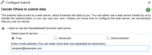
Convert your spreadsheet 
Select the output format you prefer and convert your spreadsheet to a web page with this flavor.
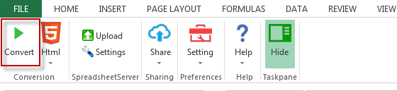
Enter data into the form and press Submit 
After conversion, the web form normally opens in one or more web browsers. If it doesn’t, open the Excel > the SpreadsheetConverter task pane > Preferences > Options > Browsers and conversion path option setting to get the name of the folder where the converted web page is stored and open the page from that folder. It is in these settings you also select one or more web browsers to open each web page automatically in after conversion.
Enter some data into the fields in the form.
While you are still offline, press the Submit button in the toolbar.

Save the form 
A pop-up will appear, asking you for permission to save the form. Click Yes and the form will be securely stored in the web browser.
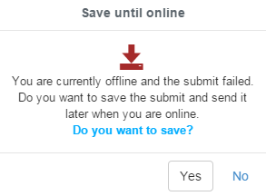
When you approve, note the new Offline Forms button that now appears in the toolbar with a counter for the number of forms saved.

Submit three more forms 
Modify the data in the form slightly and press Submit again. Notice that the counter in the Offline Forms button increases for every form you submit. Repeat this until you have queued four forms.
Go online 
Re-connect to the Internet by reversing what you did to come offline, e.g. return Firefox to online mode, re-insert the network cable, turn the data connections on your device back on, connect to wi-fi or enable the network adapter you previously disabled.
Verify that the Internet works by opening a new tab in your web browser and pointing it to www.spreadsheetconverter.com.
Submit the saved forms 
Return to the browser tab for the form you have been working with. Press the Offline Forms button in the toolbar.

Before forwarding all the saved forms to the server, SpreadsheetConverter asks you to confirm that you want to send them. Click Yes.
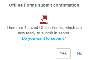
Verify the submitted forms in the Inbox 
Open the e-mail Inbox for the recipient you specified in Configure Submit. The four forms you saved in the browser while you were offline should now arrive in this Inbox.
With the Free submit service the e-mails can look a bit cryptic, we know. If you upgrade to the Advanced service the e-mails will look just like the web form, which makes them much easier to work with.
The Browser Storage Toolbar 
When you work with saved web forms there may be situations where you’d like to know more about how many forms you have saved and how much space they all occupy. If you use the Advanced Submit Service, we must also save an e-mail template to pass on to the server so that it can make each e-mail look like the submitted web form.
All these things are stored in the web browser, in something we call Browser Storage. Since most web browsers don’t provide a lot of information or tools related to Browser Storage, we have developed a simple toolbar to help you better understand what is going on with your Browser Storage. For more information, visit the help page for Browser Storage.
Help: Page fill color 
When converting for iPhone/Android, you can set a web page background color that is used for all the tabs in a form or calculator. This makes your mobile webpage look better with widgets, and maintains your corporate identity or brand color throughout a multi-page web form.
Without a page fill color, a web page can look like below. Notice the white borders around the input fields.
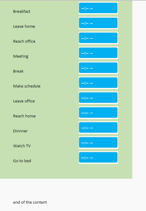
The white borders appear because the background color is derived from the Excel spreadsheet where it has to be set per cell, not for the entire page.
Setting a page fill color 
In the example, we want to use a green page fill color.
Select any cell in the spreadsheet that has the same background color as you want for the entire page, or temporarily assign the background color you want to any cell with Format Cells > Fill.
Click on the Page Fill Color setting on the Workbook tab of the task pane and select this cell to use the background color of the selected cell as the background color for all tabs in the converted web page.
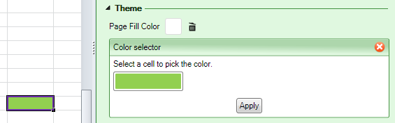
Press Apply to set the Page Fill Color. The selected background color will be applied to the entire converted web page, without regard to the separation of cells or widgets in Excel. If you assigned a temporary background color to the selected cell, you can remove it now.
Another advantage of using the page fill color is that you no longer have to assign your brand color to each tab or worksheet. Once you set a page fill color for the workbook, all tabs will have the same background/brand color.
It certainly looks a lot better without the borders!
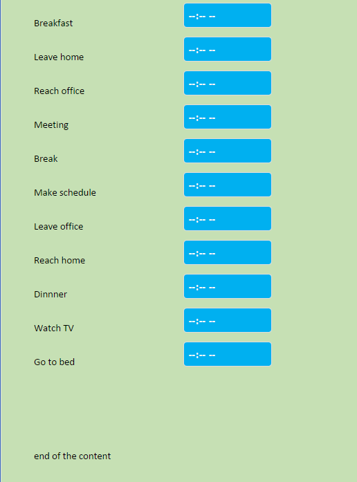
Publish to Cloud 
Publish to Cloud 
This is the online help page for the Publish to Cloud feature that uploads your web form or calculator on the web in just a few seconds.
When you have converted a spreadsheet, you want to publish it on the web. SpreadsheetConverter comes with built-in, high-performance web hosting on the globally distributed Amazon S3 infrastructure with superior performance, extreme reliability and massive scalability. Over a dozen server locations around the globe ensure that your calculator always is within easy reach of your global audience.
With Publish to Cloud, we offer 7-day test publishing for free to all our users. If you have a paid license, you can also publish calculators permanently for production purposes.
Note: If you prefer to use one of your own servers, users of WordPress can use a plugin to import spreadsheets into WordPress. If you want to upload with FTP to your own web server, there is a tutorial on how to upload forms and calculators using FTP.
Convert the spreadsheet 
Before you can upload the spreadsheet, you must convert it. It is not possible to upload an unconverted spreadsheet, or a spreadsheet that is not opened in Excel.
Select the Test or Production location 
For every spreadsheet you create, there are two upload locations: Test and Production.
You can make changes to a spreadsheet and invite other people to test it in the Test location. The Test version is automatically deleted after 7 days. If you don’t have a paid license for SpreadsheetConverter, you can only use Test links.
When testing is complete and you want to activate the new version as the live Production version, simply select to replace the Production version instead. The basic ability to create production links is included in all paid licenses except Node.js.
Production links are always the same, every time you upload the same spreadsheet, and never expire. If you wish to create an additional permanent link, e.g. for a different flavor, you need to rename the spreadsheet or a copy of it before you convert and upload the spreadsheet with the new name.
Start the upload 
- Test: Use the Test in Cloud option in the ribbon to initiate an upload of the most recently converted web page for the currently open spreadsheet to the Test location. Verify that you are uploading the most recent conversion of the spreadsheet, in the intended flavor.
- Production: When you’ve finished testing the new version, it’s time to update the production version. Use the Publish to Cloud option in the ribbon. Verify that you are uploading the most recent conversion of the spreadsheet, in the intended flavor.
Wait for the upload to complete 
While the calculator is being uploaded, a message appears in the Publish to Cloud window.
Get the link to the uploaded calculator 
After you have published the calculator to the cloud, you must save the links you get to it. We provide four different types of links:
- Full link: This is a standard web link that contains the exact server, folder and file information required for a web browser to open the calculator you just uploaded. A drawback with the full link is that it can be over a hundred characters long, which means it may not fit on a single line in an e-mail or on a web page. That is why we also offer the
- Short link: This is a typical “shortened” link in the form https:/tinyurl.com/y3otra5n. This link is much easier to use in e-mails and on web pages because it never breaks like long links sometimes do.
- QR code: If you want to publish your link in a format that is easy to use with a tablet or cell phone, you can of course use the short link above – it takes much less time to type. But why type at all? It’s even easier to click on the QR code symbol. This creates a QR code image that contains the link, then copies this image to the clipboard. All you have to do is to paste it into an e-mail or web page. Users with mobile devices simply scan the code with their camera to open the calculator on their device.
- Iframe: If you want to embed your calculator in a web page, it’s very easy to do so with an iframe. The iframe works very much like adding an image to your page, but instead of showing a static image it displays the live calculator you just uploaded. Just click on the iframe symbol to have the full HTML source code for the iframe copied to the clipboard. Then move to WordPress or whatever content management system you are using, insert a “custom HTML” block or switch to HTML edit mode and paste the HTML for the iframe into the page where you want it. Use the width and height parameters in the iframe source to adjust the size of the iframe. Below, there are links to more specific embedding instructions for some of the most common content management systems.
If you need other link formats later, just convert and upload the calculator again.
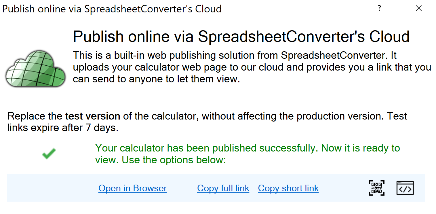
Removing an uploaded calculator 
To remove previously uploaded calculators, do the following:
- Rename the original calculator, e.g. saved_version_of_my_calculator.xlsx.
- Start Excel and create a new, empty calculator.
- In any cell, e.g. A1, insert the text “This calculator has been removed.”.
- In any other cell, e.g. A2, insert a calculation, e.g. =if(A1=””,””,””) since this is required by SpreadsheetConverter.
- Save the spreadsheet in the same folder and under the same name as the original calculator, e.g. “my_calculator.xlsx”.
- Convert the new calculator with SpreadsheetConverter.
- Upload the new version of the spreadsheet with Publish to Cloud. It will entirely replace the original calculator and display the “removed” message when someone tries to start it.
Known issues 
Usage fees and limitations 
There is currently no limit to the number of calculators and forms you may upload, or their combined size. As the use of this feature grows, we may introduce usage fees and/or limits.
Expect a small delay when you replace a previous version 
When you update an existing calculator, some advanced performance optimization techniques may retain the old version for up to 15 minutes.
Learn more 
Some of our tutorials use Publish to Cloud:
Import an Excel spreadsheet in your blog or website 
Converting spreadsheets to web format makes it very easy to import them into your blog or website. Here are tutorials on how to do this in various popular environments:
- Import Excel spreadsheets and charts in Blogger
- Import Excel spreadsheets and charts in Drupal
- Import Excel spreadsheets and charts in Google Sites
- Import Excel spreadsheets and charts in Joomla
- Import Excel spreadsheets and charts in Squarespace
- Import Excel spreadsheets and charts in Typepad
- Import Excel spreadsheets and charts in Weebly
- Import Excel spreadsheets and charts in Wix
- Import Excel spreadsheets and charts in WordPress with the plugin
- Import Excel spreadsheets and charts in WordPress without the plugin
- Import Excel spreadsheets and charts in any blog or website
Collaborate with Real-time Sync, HTML flavor 
Real-time Sync HTML 
Collaborate on a spreadsheet with anyone in the world in real-time from your web browser.
Collaborate with Real-time Sync, HTML flavor 
Use Real-time sync to share a live calculator or smart web form with other users, when the calculator has been converted for the web with the HTML flavor.
SpreadsheetConverter Real-time Sync lets you collaborate on a spreadsheet on the web. Multiple users can update the same electronic form or live calculator at the same time to make the work more efficient. In this help page, we will show you how to create a session and invite other users from a web page created with the HTML flavor of SpreadsheetConverter. There is a similar page describing Real-time Sync in the iPhone/Android flavor.
To create a session, you define a secret key for your calculator web page, then send it to your colleagues in an invitation to join the collaboration session.
Enable Real-time Sync 
In Excel, use the Workbook tab on the SpreadsheetConverter task pane to ensure that Real-time Sync is turned on for the calculator after conversion.
Convert the spreadsheet 
Open your spreadsheet in Excel. Select the HTML flavor in the SpreadsheetConverter ribbon. Convert the spreadsheet by pressing the Convert button.
Upload the spreadsheet to a web server 
Before you start collaborating on a spreadsheet, you must upload it to a web server. SpreadsheetConverter provides built-in web publishing of forms and calculators.
Open the web calculator in a web browser 
To start a collaboration session, you must first open the converted web page on the web in your web browser.
Start Real-time Sync 
Click on the Real-time Sync button in the bottom toolbar of the converted web page.

Enter a Secret key, which should be unique for each session, for your collaboration team (see the screenshot below). Use seven characters or more, preferably using a combination of letters, digits and certain special characters. For more detail, read more about the Real-time Sync security concerns.
Enter your name or e-mail address to identify you during the session. This name will be shown to the others in the session when you change field contents.
Press Connect to create the Real-time Sync session.
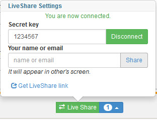
Obtain a link to the session 
Click Get Real-time Sync link. When the window to the right appears, copy the link with Ctrl + C.
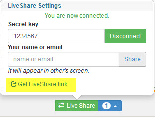
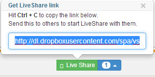
Invite other users to the session 
Share the copied link among your colleagues, e.g. by e-mail or chat.
When users enter the session, they provide the name or e-mail address they wish to use during the session.
For your convenience, the secret key is included in the link. If you wish to provide this separately, you should remove it from the link before you share it with others, by removing ?k= and all the text afterward.
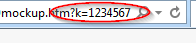
Verify that other users are connected 
Use the Real-time Sync button in the bottom toolbar to see all participants in this Real-time Sync session.

Start making changes 
As connected users make changes to the spreadsheet, a colored arrow appears with their name.
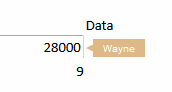
The results are always saved 
Each collaboration session is automatically saved after each change. The next time you connect to the session using the same secret key, the calculator or form will contain the values from the last time you used it.
Real-time Sync in action 
(Click the image to enlarge the video)
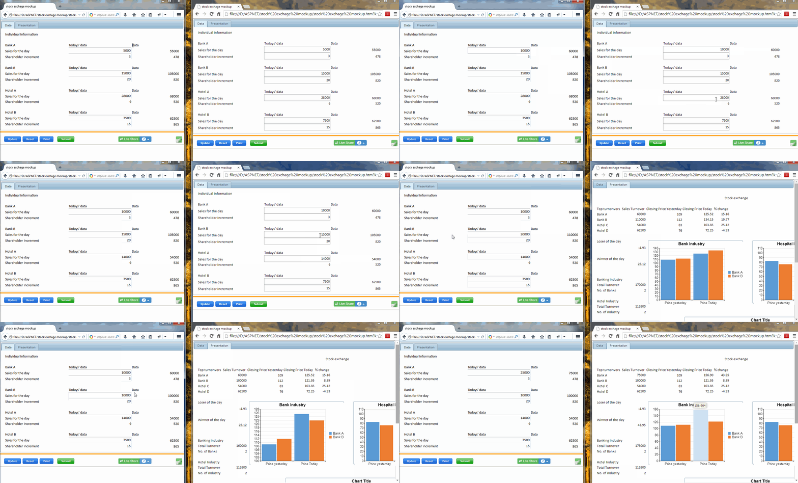
Shared web pages with saved content 
There are many ways to collaborate on an online spreadsheet. Of course, you could just use a screen-sharing program. But only Real-time Sync makes any web spreadsheet persistent, permanent, perpetual – the cloud spreadsheet is saved after every change. If you open the same spreadsheet with the same key two years later, the information you last typed into it is still there.
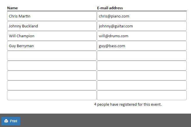
There is a detailed explanation of how you can save data in a cloud spreadsheet in the sign-up list tutorial.
Limitations 
Real-time Sync is gradually being added to SpreadsheetConverter. There are currently a few minor limitations. We hope to remove these limitations in the near future.
- SpreadsheetConverter Real-time Sync is supported in Google Chrome, Mozilla Firefox and Internet Explorer 10 and above.
- The spreadsheet must have at least one calculation or formula for Real-time Sync to work.
- The spreadsheet must have at least one button in the Toolbar.
- The Real-time Sync button can only be added to the bottom toolbar.
SpreadsheetConverter Real-time Sync Help 
Real-time Sync iPhone/Android 
Collaborate on a spreadsheet with anyone in the world in real-time from your iPhone, iPad or Android app.
SpreadsheetConverter Real-time Sync Help 
This Online Help page shows you how to use Real-time sync to share a live calculator or smart web form with other users, when the calculator has been converted for the web with the iPhone/Android flavor.
SpreadsheetConverter Real-time Sync lets you collaborate on a spreadsheet on the web. Multiple users can update the same electronic form or live calculator at the same time to make the work more efficient. In this help page, we will show you how to create a session and invite other users from a web page created with the iPhone/Android flavor of SpreadsheetConverter. There is a similar page describing Real-time Sync in the HTML flavor.
To create a session, you define a secret key for your calculator web page, then send it to your colleagues in an invitation to join the collaboration session.
Enable Real-time Sync 
You don’t have to enable Real-time Sync in the iPhone/Android flavor, since it is always on for this flavor.
Convert the spreadsheet 
Open your spreadsheet in Excel. Select the Mobile flavor in the SpreadsheetConverter ribbon. Convert the spreadsheet by pressing the Convert button.
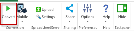
Upload the spreadsheet to a web server 
Before you start collaborating on a spreadsheet, you must upload it to a web server. SpreadsheetConverter provides built-in web publishing of forms and calculators.
Open the web calculator in a web browser 
To start a collaboration session, you must first open the converted web page on the web in your phone’s web browser.
Start Real-time Sync 
To use Real-time Sync, you first need to go to the side menu, which you open with the “hamburger” button at the top left of the screen. (If there is no side menu, you may have converted your spreadsheet with a different flavor. These instructions are for a web page converted with the iPhone/Android flavor.)
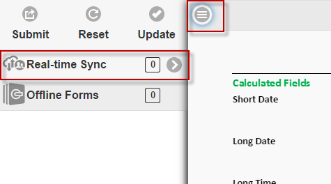
Enter a Secret key, which should be unique for each session, for your collaboration team (see the screenshot below). Use seven characters or more, preferably using a combination of letters, digits and certain special characters. For more detail, read more about the Real-time Sync security concerns.
Enter your name or e-mail address to identify you during the session. This name will be shown to the others in the session when you change field contents.
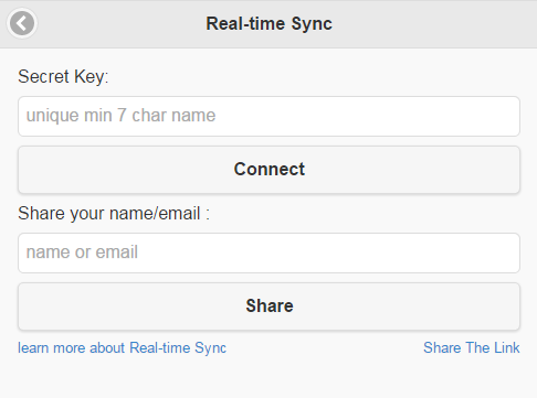
Press Connect to create the SpreadsheetConverter Real-time Sync session.
When the connect button turns green, you have successfully created a session to use Real-time Sync.
Obtain a link to the session 
Click Share the link. When the link appear above the Share the link, you can copy and share it with other participants.
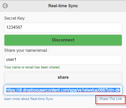
Invite other users to the session 
Share the copied link among your colleagues, e.g. by e-mail or chat.
When users enter the session, they provide the name or e-mail address they wish to use during the session.
For your convenience, the secret key is included in the link. If you wish to provide this separately, you should remove it from the link before you share it with others, by removing ?k= and all the text afterward.
Verify that other users are connected 
Use the participants button to the right in the bottom toolbar to see all participants in this Real-time Sync session.

Start making changes 
As connected users make changes to the spreadsheet, their name will appear over the field they are changing.
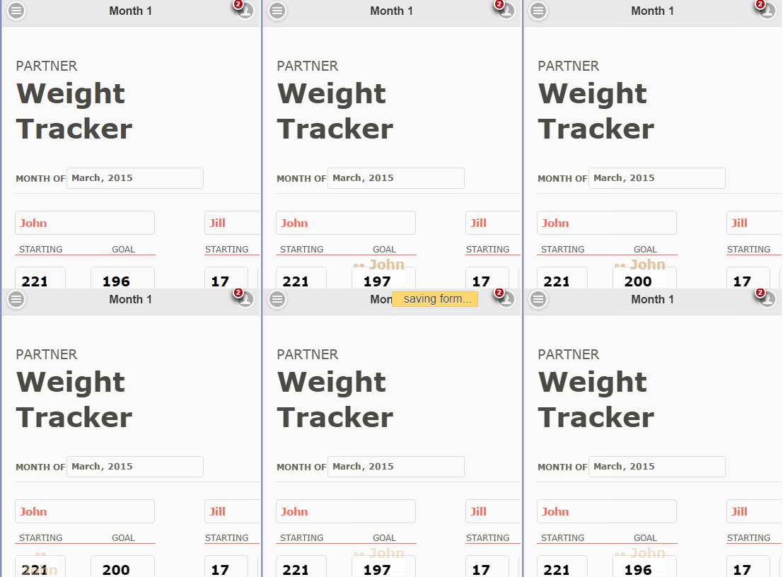
Save the results 
Each collaboration session is automatically saved after each change. The next time you connect to the session using the same secret key, the calculator or form will contain the values from the last time you used it.
Security concerns for Real-time Sync 
Security concerns for Real-time Sync 
With Real-time Sync, it is very easy to establish a collaboration session and invite other users to join in. This page describes the security concerns of sharing a spreadsheet on the web.
Once you have converted an Excel spreadsheet into a web page with SpreadsheetConverter, you can share it on the web with a feature called Real-time Sync. You may want to read the introduction to Real-time Sync before you continue.
Security concerns 
Real-time Sync was designed to provide powerful collaboration features without requirements on your existing IT infrastructure, and without requiring technical specialists. It is intended mainly for sharing of information that is of little interest to anybody else, e.g. making schedules, small budgets or for technical analysis.
To achieve this, Real-time Sync provides only rudimentary access control. If you know the link to the web page and a secret key, you’re in. For many collaboration situations, this is just the level of security you need. It’s so unlikely that someone outside the work group would 1) be interested in the results of the collaboration; 2) know the link and 3) know the secret key that this level of access control is sufficient.
Publishing business-critical information on the world-wide web is probably generally a bad idea. If you want to use Real-time Sync to collaborate on a powerful spreadsheet that documents confidential parts of your business model, pricing structure or product plans, you should seriously consider the security implications first.
Use an intranet behind a firewall 
The access control in Real-time Sync only protects the collaboration session and its saved values. The calculator itself is not protected and can always be accessed by anyone with the correct link. If you access a calculator directly without Real-time Sync, you get a single-user copy with the initial values that were in the cells when the spreadsheet was converted. If you need to control all access to the converted web page you must use the security features of the network, e.g. by using an intranet.
The servers on your intranet are located behind a firewall that makes their data less insecure. You should publish all sensitive calculators or forms only on your intranet servers, since this makes it almost impossible for someone on the outside to access them.
Consider using a protected folder 
It is usually very difficult to keep a web page completely secret. Many publishing systems indirectly link to all pages they publish, making it easy for an indexing spider to add the page to its index and possibly even making the calculator searchable. Most spreadsheets contain a lot of text that an indexing spider will save in its index, making it easy for anyone behind the firewall to find your spreadsheet if they use the right search terms.
To avoid prying eyes it may be useful to save the calculator in a reserved folder that is only available to approved users. Once again this is standard network access control and has nothing to do with Real-time Sync.
Make the secret key secure 
The secret key used by Real-time Sync provides an extra level of security for the collaboration session and its saved data. Even if you have access to the calculator itself, you cannot participate in the collaboration session unless you know the secret key. If the Real-time Sync session itself is sensitive, you should use a secret key that is long, with a combination of letters, digits and special characters that is impossible to guess.
Since the secret key is used in the “k” parameter of the link to the calculator, it must conform to the rules for what characters links may contain. If you want to use special characters in your secret key, you can safely use only the following, since they have no reserved meaning in a link:
$ dollar sign
- minus sign or hyphen
_ underscore
. period
+ plus sign
! exclamation point
* asterisk
' apostrophe
( left or opening parentheses
) right or closing parentheses
, comma
Send the secret key separately, not in the link 
If you include the secret key in the link you send to your collaborators, you make it much more convenient for them to directly access the shared session, but if any possible intruders find the full link, they also have full access the shared session:
http://www.example.com/budget/budget.htm?k=northwest
Instead of sharing the full link with your collaborators, you should only send them the safe, plain link:
http://www.example.com/budget/budget.htm
and then separately provide them with the secret key northwest that they need to join the sharing session by pressing the Real-time Sync button in the toolbar and manually entering the secret key.
Using the secret key as a session name 
If you want to use the same calculator as a template for more than one Real-time Sync session, e.g. for different time periods, geographical regions or market languages, you must use a different secret key for each session. To make it easier for users to handle the increasing number of keys, consider including things like months or region names in the secret key.
Example: You have decided to use the secret key “Internat10nalHarve$ter”, since it is pretty easy to remember but very difficult to guess. To use this secret key for the January figures for the French-speaking markets of Europe, you may use the combined secret key “Internat10nalHarve$ter-EU-FR-Jan”. Since all combinations of market, language and month create their own collaboration session, it is easy to keep each session separate.
Help: Tips and tricks for web forms and submit 
Forms tips and tricks 
Here are some nice things to know about electronic forms and the submit process.
When you create electronic forms with SpreadsheetConverter, there are a few special features that we describe in this document.
You can build web forms that automatically get sent to your e-mail Inbox every time someone uses the form. For a small monthly fee, you can also have each submitted form stored in a hosted database for later retrieval. Read more about our Free and Advanced Submit Services.
Use Required fields 
You don’t want to receive forms where vital information is missing. Most widgets have a Required option. If you select this option for the widget, it will not be possible to submit the form without providing information in the field.
Validate as much as you can before submit 
You don’t want to receive forms where the information is incorrect. SpreadsheetConverter supports most of Excel’s Data Validation features. Use these to validate as much as you can of every field in the form. This makes it impossible to submit the form if it has any known error.
- Verify that each field has the right kind of content, like an integer, a date or a correct e-mail address.
- Ensure that each field has a value within the expected range, e.g. 1-5.
- Require text fields to be of a certain length.
- Provide only a fixed set of options for a field.
- Use an Excel formula to validate the contents of a field.
Use locked or hidden fields 
You normally don’t need to lock cells that you don’t want your users to change. By default, the cells in your spreadsheet do not become open for user input when the spreadsheet is converted into a web form. There are three different ways to unlock a cell for input. If you don’t use either of them, users will see the cell contents but will be unable to change them. Read more about designating input cells.
To completely hide a cell’s contents from the user, place a Text or Utility widget in the cell and tick its Make hidden field check-box.

Use named cells as input fields 
You should always assign names to your input fields, i.e. the cells that you will open for input from the user. This makes it much easier to decode the electronic form later. With the Advanced Submit Server, the cell name is used as the field name when you browse through the submitted forms in the Advanced Server, and as the column name when you download them.
You assign a name to a cell using Excel’s naming mechanism or by using the Name field of any widget.

Send the form to the Form Recipient 
When you create a web form, you must decide what should happen when the submitter presses the Submit button in the form. If you use our Free or Advanced Submit Service, the form’s contents are sent in an e-mail to a predefined e-mail address that we call the Form Recipient. You set this address in the form’s Submit options.

Note that you cannot change the From address for the e-mails containing form submissions. All these e-mails are sent from our servers and the e-mail infrastructure does not appreciate that we send e-mail pretending to be from someone else.
Send a copy of the form to the Form Submitter 
We can also automatically send an additional copy of the form to the person that submitted it. We call this the Form Submitter e-mail address – but you can actually use any valid e-mail address for this second copy of the submitted form.
To activate this feature, give a cell in the spreadsheet the reserved name email (without the hyphen) and provide a second e-mail address there.

If you wish to assign a particular subject to this message, give a cell in the spreadsheet the reserved name subject and provide a text for the e-mail Subject there.

If you are uncomfortable using the shorthand notation with the named cells, you can activate the same feature using the Configure Submit settings on the Workbook tab.
The e-mail address and the optional subject for this e-mail can be provided in several ways:
- Before you convert the spreadsheet to a web page, type a static e-mail address and subject into the cells named email and subject in the spreadsheet.
- Provide the e-mail and subject directly from the form’s contents in cells with the reserved names email and subject.
- You can concatenate values from more than one form field using Excel’s & string operator like in the example above.
- You can use advanced conditions in Excel IF clauses.
- You can use a formula like VLOOKUP to dynamically assign text depending on other values in the form.
- If you are comfortable handling URL query strings and know the technical requirements for doing this, the email and subject cells can be set from the form’s URL like any other named cell. This allows you to set these values directly in the link to the form sent to the submitter, or from a script. Example:
http://example.com/form.htm?email=x@y.z&subject=Application
In some of these situations, you may want to hide or lock the cells (see above) so that the Submitter doesn’t see or change them.
Note that you cannot change the From address for the e-mails containing form submissions. All these e-mails are sent from our servers and the e-mail infrastructure does not appreciate that we send e-mail pretending to be from someone else.
Sending e-mails between Form Submitter and Form Recipient 
When a form contains an email field, it becomes easy for the person that submitted the form to communicate with the recipient, and vice versa.
- If the Form Recipient replies to the received form, the reply is sent to the Form Submitter e-mail address. This makes it easy for the recipient to follow-up on form submissions and ask additional questions.
- If the Form Submitter replies to the e-mail with the submitted form, this response is sent to the Form Recipient. This makes it easy for the submitter to provide additional information.
For faster submits, use the index-quick.htm file 
If you use the Advanced submit service, we recommend that you use the “light” index-quick.htm file for all submissions of the form except the first. The index-quick.htm file is often much smaller than the full web form which can save time when users download and submit the form. If your users need to submit the form while they’re offline, you may even be forced to use this leaner version of the form to pass the size requirements.
Before you enable the index-quick.htm page, ensure that you have submitted the “full” form at least once, to allow it to be saved on the forms processing server. Whenever you make changes to the appearance of a form you must submit the full form at least once again, to update the copy in the server.
Translate the texts 
You can translate or edit the messages that are issued during form submissions, e.g. “The form was successfully submitted.” Read more in the help for Submit.
How do I design a spreadsheet to look good as a web page ? 
Read our comprehensive design guide to learn how to design web calculators for a global, mobile audience:
- A large part of your users will be using their phones to use the web page.
- Put the caption on top of each field, not to the left of it.
- Arrange the sections of the calculator or form below each other, or on different tabs.
- For wider examples, you must use responsive design to make the example fit also narrow screens.
- As a desktop user, you may love to analyze data in wide tables with countless columns. This doesn’t work well on phones. You have many options.
- Always test all your calculators with your own phone.
- Assume your calculator or form will be used by an international audience.
- Your calculator may need to handle both metric and US customary units.
- Learn more about the differences in the formatting of date, time and numbers.
- Use only colors that are as far away from each other as possible, using colors that are unambiguous also to colorblind persons.
- Use the table in the design guide.
Try this Excel add-in now! 
Click on Download to install and test this Excel add-in for Windows.
Click on Upload to let us convert a spreadsheet for you for free.
Help: Use the basic widgets, iPhone/Android flavor 
SpreadsheetConverter offers you lots of basic graphical widgets that make your web page easier to use and to give it a better appearance. This is the online help page for many of these widgets.
This is an introduction to the use of widgets in spreadsheets to improve the functionality and appearance of the converted web page. If you haven’t used widgets before, you may want to read the Introduction to using widgets before you continue.
Be aware that most of these widgets have no corresponding representation when used in Excel. Some of them are unfortunately totally invisible in Excel. You have to convert the spreadsheet to web format to see the widget in action.
This page describes the widgets available in the iPhone/Android flavor. There is a similar page describing the widgets in the HTML and Node.js flavors.
Text 
Text fields are mainly used in electronic forms to mark the fields where the user will enter data that is not used in calculations, e.g. a name or an address. You insert a Text field widget by clicking the Text widget in the Widgets tab in the task pane.
e”>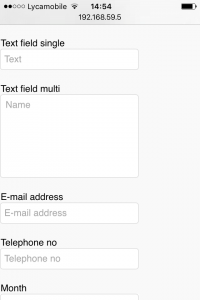
You can then set different properties for the Text field:
- A Required field requires input from the user. This option is mainly used for electronic forms, where a form must contain a minimum of information to be meaningful. For Text fields, a Required field cannot be empty. If it is, it will not be possible to submit the form.
- Make hidden field is used when you want a cell to be visible in the spreadsheet, but not in the converted web page. This also allows you to provide information to a form processing script without showing it in the form. As an example, if the link to the form contains a language code (/form.htm?lang=sv), it will be preserved by the form if your form has a text field named lang, and it will be forwarded with the form when the form is submitted for processing. Read more about filling form fields from the link.
- Multiline is used to give a text area more than one line and to make it scrollable. Use this option only for text fields that you have made sufficiently large in the spreadsheet, e.g. by merging two or more cells. You can achieve the same result by enabling Wrap Text for the merged cell in Excel.
- Placeholder can contain a text prompt for the field that is visible in the field only when it is empty. As an example, the Placeholder field itself displays the placeholder enter label or hint until you type anything into the field.
- Name your widgets if you want to pass data into them from the link to the form (see above). For electronic forms, it is also much easier to process the form if all input fields have names. You can name your fields in the widgets or give them cell names in Excel. Widget names can start with numbers or an underscore, which is required when integrating with products like Salesforce.
- The default value of a Text field is empty. To provide a different default value, enter text into the spreadsheet cell before conversion.
Learn more 
Some of our tutorials partly focus on the Text widget:
Email, Telephone, Month, Week, Number 
Special widgets for small touchscreens 
When using a mobile device, it can sometimes be difficult to enter data with proper formatting. Many mobile devices offer optimized keyboards for special data types, e.g. a numeric keypad. Some browsers offer data entry templates like date pickers, and even provide syntax validation.
SpreadsheetConverter provides special touchscreen widgets request that the user’s web browser provides additional assistance when entering certain types of input. Your mobile users will be grateful for this help.
The browser provides the user assistance 
A word of caution, though: Although we can request this assistance from the browser, we cannot guarantee that the browser properly supports all input types, or that your users appreciate the help the browser is trying to provide. As an example, the full syntax for an e-mail address is very complicated and you can expect most web browsers to reject unusual but formally correct e-mail addresses such as john.smith(My Johnny!)@example.com or john.smith@[IPv6:2001:db8::1] while cheerfully approving obviously incorrect e-mail addresses such as john.smith.@example.com.
Users don’t like having correct input data flagged as incorrect by poorly tested web browsers. If possible, please test the advanced input types carefully before you implement them.
Examples of touchscreen widgets 
- E-mail address – “.com” and other top level domains may be added to the keyboard by the browser, and the e-mail address may be validated for proper syntax.
- Telephone number – a special telephone keyboard may be provided by the browser, and the field contents may be validated.
- Month – a date picker for year and month may be provided by the browser in the default language and regional format set for device.
- Week – a date picker for year and week may be provided by the browser in the regional format set for device.
- Number – a numeric keypad may be provided by the browser, and non-numeric content in the field may be flagged.
- Date – a date picker may be provided by the browser in the default language and regional format set for device.
- Time – a time picker may be provided by the browser in the regional format set for device.
Properties for the touchscreen widgets 
The properties for the touchscreen widgets are the same as for the Text widget. Read more above!
Slider 
A Slider allows the user to select a value by moving a handle to a particular position on the widget. Sliders are real-time and cause the entire spreadsheet to be continuously recalculated with each new value of the slider as you move it.
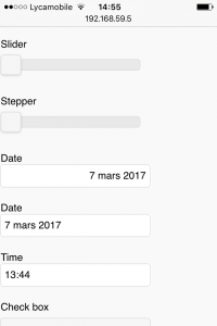
You insert a Slider widget by clicking the Slider widget (value increases from left to right) in the Widgets tab in the task pane.
- The Minimum value is the value the widget returns at the slider’s leftmost or bottom position, depending on its orientation.
- The Maximum value is the value that the cell contains when the slider is in its top or rightmost position, depending on its orientation.
- Use the Tick Interval if you want tick marks along the slider.
- Name your widgets if you want to pass data into them from the link to the form (see below). For electronic forms, it is also much easier to process the form if all input fields have names. You can name your fields in the widgets or give them cell names in Excel. Widget names can start with numbers or an underscore, which is required when integrating with products like Salesforce.
- The default value of a slider is whatever value you put in the spreadsheet cell before conversion, or the minimum value.
- You can assign a value to a slider widget from the link. Use the format /form.htm?example=42. Read more about filling form fields from the link.
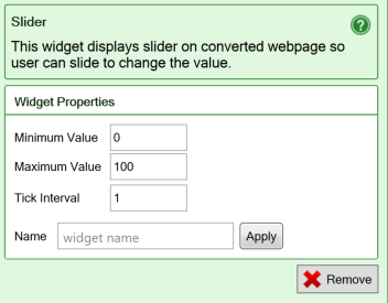
Learn more 
Some of our tutorials partly focus on the Slider widget:
Stepper 
The Stepper widget allows you to easily input small numeric values with just a tap or click on a button.
The worksheet is re-evaluated for each new value, making this a very useful widget when the user is trying to find an optimum value.
- The Minimum value is the lowest value the widget can have. The minus button stops working at the minimum value.
- The Maximum value is the highest value the widget can have. The plus button stops working at the maximum value.
- Use the Tick Interval if you want the step to be different from 1.
- Name your widgets if you want to pass data into them from the link to the form (see below). For electronic forms it is also much easier to process the form if all input fields have names. You can name your fields in the widgets or give them cell names in Excel. Widget names can start with numbers or an underscore, which is required when integrating with products like Salesforce.
- The default value of a stepper is is whatever value you put in the cell, or the minimum value.
- You can assign a value to a stepper widget from the link. Use the format /form.htm?example=2. Read more about filling form fields from the link.
Date picker and Time 
The Date Picker and Time widgets make it much easier for the user to pick the right date and time. The widgets ensure that any date or time set in the widget is valid, and formats it correctly for the recipient of the electronic web form using the regional settings.
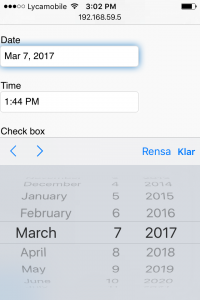
Date picker 
The default value of a date picker widget is the current date. The Date will be formatted according to your computer’s regional settings.
- Name your widgets if you want to pass data into them from the link to the form. As an example, if the link to the form contains an Excel serial day number (/form.htm?date=20376), it will be preserved by the form if your spreadsheet has a cell named date, and it will be forwarded with the form when the form is submitted for processing. Read more about filling form fields from the link. For electronic forms it is also much easier to process the form if all input fields have names. You can name your fields in the widgets or give them cell names in Excel. Widget names can start with numbers or an underscore, which is required when integrating with products like Salesforce.
Time 
The default value of the Time widget is empty. The Time will be formatted according to your computer’s regional settings.
The properties for the Time widget are the same as for the Text widget. Read more above!
Link Image 
Save all relevant image links in your spreadsheet or create formulas that can build the right image link dynamically from user input.
Use the Link Image widget to select the image that is shown.
Google Map widget 
The Google Map widget allows you to use interactive maps in the converted web page.
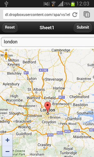
Barcode widget 
Use the barcode widget to display a barcode from static or calculated content in your web form.
Check box 
Use check boxes only for statements that must be either true or false, there is no room for doubt, like “British citizen”. The Toggle switch allows you to use any two other names for True and False, e.g. a language pair.
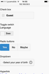
Touch checkbox 
You insert a Check box widget by clicking the Check box widget in the Widgets tab in the task pane. A Check box will provide a true/false value that you can test for in other places in the form, or when the form is submitted for processing.
- A Touch Checkbox looks like the check mark in the widget’s icon, with a label to the right.
- The Label for a Touch Checkbox contains a descriptive text, like “British citizen”, so people know when to check the box or not. Clicking on the label will also check/uncheck the check box, providing a larger touch surface on touch screens.
- After you’ve converted the spreadsheet to a web page, the label appears to the right of the check-box. Unfortunately, the label you set here cannot be shown in Excel.
- When you add a Touch Checkbox to a spreadsheet, it is initially set to FALSE. When you convert the spreadsheet to a web page, a Touch Checkbox widget will therefore initially be unchecked. If you change the default value by typing TRUE into the widget’s spreadsheet cell before conversion, the Touch Checkbox will be checked when the page is opened in a web browser.
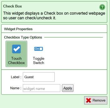
Toggle Switch checkbox 
- With a Toggle Switch check-box, the Label will appear above a small graphic that is intended to resemble an electric switch. Users can drag the handle or tap one side of the switch to toggle the check-box.
- When you flip the switch to the right, it returns a TRUE value. Flip it to the left and it sets a FALSE value for the cell.
- A Toggle Switch has three labels: one that shows what the switch does and one for each state. You can use up to four characters for the On Label and Off Label, like On/Off or Yes/No. The On Label is visible in the switch when the value of the cell is TRUE and the switch is flipped to the right.
- Only the selected state is visible in the widget, e.g. Show. Your users will assume that flipping the switch will set the opposite state, e.g. Hide.
- When you add a Toggle Switch check-box to a spreadsheet, it is initially set to FALSE. When you convert the spreadsheet to a web page, a toggle switch will therefore initially show its Off Label, flipped to the left. If you change the default value by typing TRUE into the widget’s spreadsheet cell before conversion, the check-box will be flipped to the right and show its On Label when the page is opened in a web browser.
- Note: a cell containing a Toggle switch always returns TRUE or FALSE. It does not contain the text from the On Label or Off Label. If you need this function, use a Radio button instead.
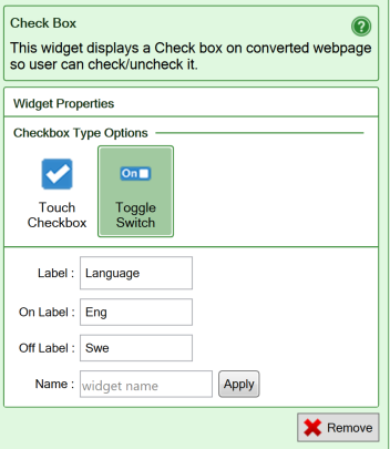
Common settings 
- Name your widgets if you want to pass data into them from the link to the form (see below). For electronic forms, it is also much easier to process the form if all input fields have names. You can name your fields in the widgets or give them cell names in Excel. Widget names can start with numbers or an underscore, which is required when integrating with products like Salesforce.
- You can set the value of a checkbox widget from the link. Use the format /form.htm?example=TRUE. Read more about filling form fields from the link.
Radio button 
Radio buttons simulate the behavior of old car radios. When one of the buttons is pressed, the corresponding radio station (option) is selected. Simultaneously, all the other buttons pop out, leaving only the selected button in the pushed-in position.
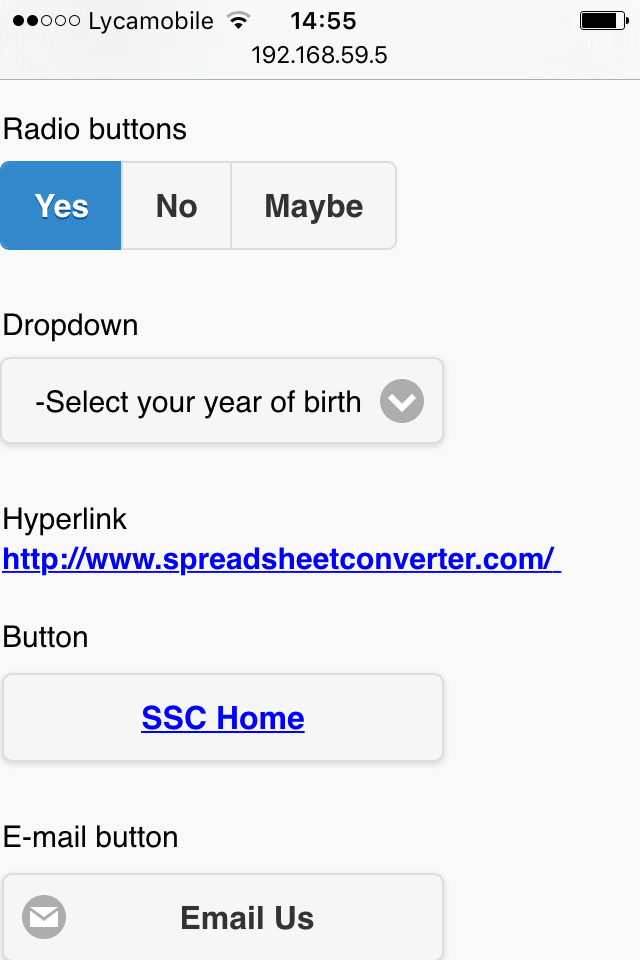
Radio buttons are used to select between a limited number of choices. The good thing about radio buttons is that you see all the available choices. The bad thing is that this may consume a lot of screen space. You insert a Radio buttons widget by clicking the Radio Button widget in the Widgets tab in the task pane. You can then set different properties for the Radio button widget:
- A Required field requires input from the user. This option is mainly used for electronic forms, where a form must contain a minimum of information to be meaningful. For Radio buttons, one of the buttons must be “pressed”. If no button is selected, it will not be possible to submit the form.
- Button labels are the names for each button. You get one button for each label you enter.
- In a Vertical Layout, the buttons are aligned in a column.
- In a Horizontal Layout, the buttons are aligned in a row.
- Name your widgets if you want to pass data into them from the link to the form (see below). For electronic forms, it is also much easier to process the form if all input fields have names. You can name your fields in the widgets or give them cell names in Excel. Widget names can start with numbers or an underscore, which is required when integrating with products like Salesforce.
- The default value of a radio button is the first choice on the list. To provide a different default value, move one of the other choices to the top of the list.
- You can select an option in the radio button from the link. Use the format /form.htm?example=Banana. Read more about filling form fields from the link.
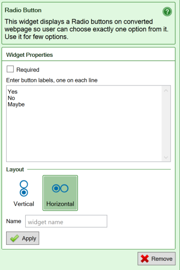
Dropdown 
Drop-down lists are used to select between a limited number of choices. The menu opens when you click on it. When you have made your choice, only the selected choice is visible.
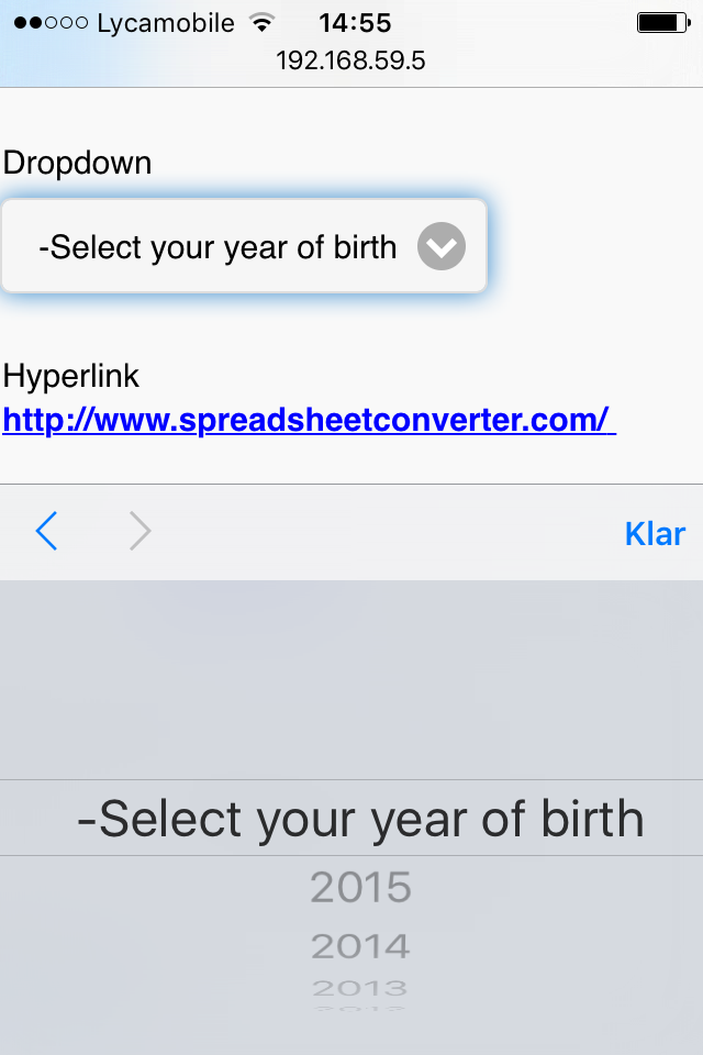
You insert a Dropdown list widget by clicking the Dropdown List widget in the Widgets tab in the task pane. List the labels in each line in the empty space. You can then set different properties for the Dropdown List:
- A Required field requires input from the user. This option is mainly used for electronic forms, where a form must contain a minimum of information to be meaningful. For Drop-down lists, the user must move the menu away from the option that is selected by default. If the default option is left selected, it will not be possible to submit the form.
- Show default text instructs the widget to add a dummy choice at the top of the list that implies that no “real” option has been selected yet – typically it’s is also used as a prompt, as in
“Rate the course, 4 is the best”. - List labels are the possible choices in the menu.
- Name your widgets if you want to pass data into them from the link to the form (see below). For electronic forms, it is also much easier to process the form if all input fields have names. You can name your fields in the widgets or give them cell names in Excel. Widget names can start with numbers or an underscore, which is required when integrating with products like Salesforce.
- The default value of a drop-down list is the first choice in the list. To provide a different default value, move one of the other choices to the top of the list.
- You can select an option in the dropdown widget from the link. Use the format /form.htm?example=Banana. Read more about filling form fields from the link.
- The basic Dropdown widget can only have one static list of choices. If you need a multi-level menu structure, e.g. select country then city, or want to prepare the list of choices with formulas in the spreadsheet, use the Dynamic Dropdown widget instead.
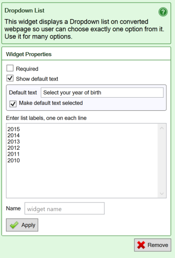
Dynamic Dropdown 
If you want the options in a dropdown menu taken from cells in the spreadsheet, learn more about the Dynamic Dropdown widget.
Hyperlink and Button 
The Hyperlink widget allows you to easily insert links into the converted web page, either as text links or as buttons.
Any cell in your worksheet can contain a web address in the form of a Universal Resource Locator or URL:
Notice that Excel considers this to be just plain text. Nothing will happen if you click on this cell. If you convert this spreadsheet to a web page, the URL is generated as plain text there too, and clicking on it will have no effect.
To turn a URL into a working link, you have to insert a hyperlink into the cell. You can let Excel create a hyperlink automatically every time you enter a URL into a cell, or you can use the Insert Hyperlink command:
Notice that the Text to display in the link, often referred to as the link’s anchor text, can be different from the link’s Address. You can usually see that a cell contains a hyperlink anyway, because of its classic formatting in blue with an underline:

By default, SpreadsheetConverter preserves hyperlinks on the converted web page. The anchor text will be displayed and linked to the requested URL.
A link in Excel can also be calculated with the
=HYPERLINK(Address, Text to display)
function. In this case the Address portion of the link is assembled dynamically according to the formula you have specified. The URL may be determined conditionally using the IF function or the address assembled from other cells. The Address to use in a given situation can even be selected with the VLOOKUP function from a list of links. The Text to display operand of the Hyperlink function allows you to define the anchor text for the link.
The Hyperlink widget in SpreadsheetConverter provides a few additional useful features:
- A Style setting that allow you to present the link also as a button, either in the cell or in the SpreadsheetConverter toolbar. The link’s anchor text will be used on the button. The design of the button can be modified by a theme.
- A Placement setting where you currently only can specify that you want the link or button to be placed in the currently selected cell.
- An Open In setting that lets you specify how you want the linked page to open: in the same browser tab, in a new browser tab, in the same frame of the web page or in the parent frameset. In the generated HTML, this selection is reflected in the HTML target parameter for the link, which will be omitted, set to _blank, set to _self or set to _parent, respectively.
- Name your widgets if you want to pass data into them from the link to the form (see the Text field widget above). For electronic forms it is also much easier to process the form if all input fields have names. You can name your fields in the widgets or give them cell names in Excel. Widget names can start with numbers or an underscore, which is required when integrating with products like Salesforce.
Email button 
An E-mail Button converts to a mailto (“send an e-mail to this e-mail address”) hyperlink. When the button is pressed, the default e-mail client normally opens a new, empty e-mail with the provided e-mail address as the e-mail recipient. The user enters the Subject and Text for the e-mail, then clicks Send to send the e-mail.
Note that none of this functionality is provided by SpreadsheetConverter. It is up to the user’s web browser to handle mailto links. If the user’s web browser is not properly configured to handle mailto links, the results are unpredictable.
The contents of your web form or calculator will not be involved in the processing started by the E-mail Button widget. If you wish to submit the full contents of a form or calculator, configure the web form’s submit options.
- Enter the recipient’s e-mail address in the Mail To field. The From field of the new e-mail will normally be set automatically by the e-mail client. All other fields of the new e-mail will be empty.
Call Button 
A Call Button converts to a tel (“initiate a telephone call to this number”) hyperlink. When the button is pressed, the device will initiate its normal behavior for tel hyperlinks, which usually is to make a telephone call to the number you have specified.
Note that none of this functionality is provided by SpreadsheetConverter. It is up to the user’s web browser to handle tel links. If the user’s web browser is not properly configured to handle tel links, the results are unpredictable.
The contents of your web form or calculator do not participate in the processing started by the Call Button widget, and nothing is sent to the designated telephone number.
- Enter the number you want the device to call in the Tel No field. The telephony infrastructure may require that you provide the phone number in a specific format. We recommend that you provide both country and area codes to ensure that the telephone number always works, regardless of the user’s location. The telephony infrastructure will usually also provide a Caller ID, i.e. the telephone number that the call originates from.
Action Buttons 
The Submit, Update and Reset buttons are the standard action buttons in your iPhone/Android calculator. That’s why we put them on the most accessible place – at the top of the Side Menu. Touch the “hamburger” in the upper left-hand corner and you see them.
However, sometimes you may want to place an action button elsewhere, perhaps to simplify the user interface. Using widgets, action buttons can be inserted in any cell in the calculator.
The text of all buttons can also be changed. Just type the text you want on the button into the cell where you place the widget.

Submit Action button 
The Submit button send the form to a web server for processing. Insert a Submit button at the end of your long form to save your users from having to scroll back to the top to reach the Submit button in the Side Menu.
Update Action button 
For smaller calculators, SpreadsheetConverter automatically updates all cells in a spreadsheet if one of the values is changed, just like Excel does. For a very complex web calculator, you have the option of switching to manual updating of the calculator in the Recalculation method setting on the Workbook tab. In that case, an Update button is needed to manually initiate the updating of the spreadsheet.
You can now place also the Update button in any cell, perhaps right after your most popular input fields.
Reset Action button 
The Reset button clears all input fields in a form. It is rarely used, except in situations where a large number of fields contain values that never will be re-used. You can now make the Reset button available where-ever users need it.
Print action button 
SpreadsheetConverter supports three printing operations:
- Print All – prints all worksheets separately.
- Print This – prints the current worksheet.
- Print – prints the print sheet if there is one, or the current worksheet.
If you initiate the print operation from the web browser with the Print menu option or the Ctrl-P keyboard shortcut, it corresponds to the Print operation in the list above.
For each Print operation, there is an action button that you can insert into any cell in the spreadsheet.
Hide Rows/Sheets widget 
You can hide certain rows in your spreadsheet, and even entire worksheets, depending on the contents of a controlling cell.
File Attachments widget 
If your users want to include files with their form submissions, e.g. a CV with a job application or an image with an error report, add a File Attachments widget to your form.
Utility 
The Utility widget can be used to assign a name to a calculated cell, or to make it invisible.
You insert a Utility widget by clicking the Utility widget in the Widgets tab in the task pane. Utility cells in a form or calculator are always locked for user input in order to preserve the contents
- Make hidden field is used when you want a cell to be visible in the spreadsheet, but not in the converted web page. This also allows you to provide information to a form processing script without showing it in the form. As an example, if you use a cell to keep track of how long it took a user to fill in a form, you may want to hide this calculation. Even though the field is hidden, it is forwarded with the form when the form is submitted for processing.
- Name your widgets in electronic forms since it becomes much easier to process the form if all input fields have names. You can name your fields in the widgets or give them cell names in Excel. Widget names can start with numbers or an underscore, which is required when integrating with products like Salesforce.
- Utility cells get their default values from the formulas in the cell.
Learn more 
Some of our tutorials partly focus on the Utility widget:
Troubleshooting 
Troubleshooting 
Follow these instructions to troubleshoot technical problems with SpreadsheetConverter.
Do you have problems downloading and installing the add-in? Are you using the add-in but it doesn’t work as you expect? Just follow the steps below and we will help you make it work.
If you have problems during download and installation 
If you have installed SpreadsheetConverter but there is no SpreadsheetConverter tab in your Excel ribbon, or if you have problems related to download or installation, follow the instructions on the help page for download and installationr.
Check the Known Issues 
The problem you have may already have been detected by or reported to us. Until we can fix such issues, we document them on the Known Issues page.
If you use offline forms, the old offline forms feature was built on a web standard called AppCache that is now being deprecated. Read more on the help page for offline forms.
Verify you have the latest version of the add-in 
The problem you are experiencing may already have been solved in the most recent update of the add-in. Before reporting a problem, you should always open the About box from the ribbon.
The About box will alert you if you should download and install the latest update of the version covered by your SpreadsheetConverter license.
Test with one of our examples 
If the converter does not work as you expect, e.g. it stops during conversion or you get strange messages from Windows, Excel or the add-in, this may or may not relate to the actual spreadsheet you are converting. To make it simpler for our help desk to recreate your problem, please use the Try Examples link in the ribbon to open the Weekly Time Card example that was installed with SpreadsheetConverter.
The example spreadsheet does the following:
- It verifies that add-in was installed correctly and is available in Excel.
- It runs a test conversion of the example spreadsheet to a web page.
- It opens the converted web page in your default web browser.
If any of these steps fail, please uninstall the program from Settings > Apps and install it again.
If you still get the same problem you had before, it is better for us if you report it against our example than your own spreadsheet that we don’t know anything about.
Report technical issues inside the add-in 
If you are working with a spreadsheet and not getting the results you want, or if you get error messages that you don’t understand, it is always best to use the Report Issue function in the add-in. This ensures that our help desk gets all the logs and system info they may need to understand the problem. Just click on the button in the SpreadsheetConverter ribbon and fill in the form.
If the Report Issue function doesn’t work, please use the contact form instead.
Use the Contact Form 
If you need help, describe your problem using the Help Desk contact form.
You’re not alone 
We provide the best possible support, both for trial users and customers.
User-defined functions 
User defined functions 
User-defined functions help you with the calculations that Excel doesn’t support.
User-defined functions 
SpreadsheetConverter does not support Excel macros, but you can manually convert your macros to JavaScript and use them in the converted web page.
SpreadsheetConverter supports Excel formulas and about 300 Excel functions. Macros written in Visual Basic for Applications (VBA) are not automatically converted and included with the web page.
However, if you can translate these functions to JavaScript yourself, the generated code can call them.
In the spreadsheet udf_toy.xls you can see the signature of the three functions that can be user-defined. The functions will be called each time the spreadsheet is recalculated.
Our implementation is currently limited to three user-defined functions per spreadsheet. If you need more flexibility, you can use the first string argument to request the sub-function, e.g. “find-insert”, “find-replace”, “find-delete”, and have a switch in your code to run the code that handles each sub-function.
Our recommendation is that you define the functions twice, once in Excel for testing, and then in JavaScript for implementation.
You have to manually paste the definitions into the HTML created by SpreadsheetConverter every time you convert the spreadsheet. Please contact our Help Desk if you need help defining user functions.